Identifying and extracting numbers for the Sudoku OCR Reader.

Update 5 August 2023: code refactoring.

This post is part of a series. The other articles are:

All code is available online at my repository: github.com/LiorSinai/SudokuReader-Julia.

Part 3 - digit extraction

Straightening the image.

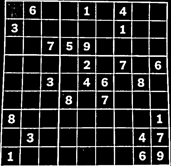
From part 2 we have a quadrilateral which represents our grid. We could mask our image to exclude pixels outside the quadrilateral and crop it to the rectangle borders. For example:

But we can do one better: we can straighten the whole grid. While the grid extraction from the previous section might have been done with machine learning, I don’t think this straightening can be.

PyImageSearch has a great Python tutorial on how to do this. I’ve recreated the code and their explanations here in Julia. It was slightly harder than using OpenCV in Python because I had to write more of the functions myself.

Firstly our points should be in a consistent order. This is so that we map the top-left point of the quadrilateral to the top-left point of the rectangle and so on. As a sanity check, we can do the following:

function order_points(corners::Vector{<:CartesianIndex})
	# order points: top-left, top-right, bottom-right, bottom-left
	rect = zeros(typeof(corners[1]), 4)
	# the top-left point will have the smallest sum, whereas the bottom-right point will have the largest sum
	s = [point[1] + point[2] for point in corners]
	rect[1] = corners[argmin(s)]
	rect[3] = corners[argmax(s)]
	# now, compute the difference between the points, the top-right point will have the smallest difference,
	# whereas the bottom-left will have the largest difference
	diff = [point[2] - point[1] for point in corners]
	rect[2] = corners[argmin(diff)]
	rect[4] = corners[argmax(diff)]
	# return the ordered coordinates
	return rect
end

Next we calculate a four point transformation matrix that will transform our four quadrilateral points to four rectangular points. We can use fit_rectangle from part_2 to get our destination rectangle. We can use warp from ImageTransformations.jl to apply the matrix to our image.

using ImageTransformations, CoordinateTransformations
using StaticArrays

function four_point_transform(image::AbstractArray, corners::Vector{<:CartesianIndex})
    quad = order_points(corners)
    rect = fit_rectangle(corners)
    destination = [CartesianIndex(point[1] - rect[1][1] + 1, point[2] - rect[1][2] + 1) for point in rect]
    maxWidth = destination[2][1] - destination[1][1] 
    maxHeight = destination[3][2] - destination[2][2] 

    M = get_perspective_matrix(quad, destination)
    invM = inv(M)

    warped = warp(image, perspective_transform(invM), (1:maxWidth, 1:maxHeight))
    warped, invM
end

We need to return the inverse matrix because it is needed for projecting text back on to the grid, which we will do in part 5. The function get_perspective_matrix is detailed in the more detail block below.

I’ve built the perspective_transform function with the function composition notation of CoordinateTransformations.jl as follows:

extend1(v) = [v[1], v[2], 1]
perspective_transform(M::Matrix) = PerspectiveMap() ∘ LinearMap(M) ∘ extend1

It is mathematically equivalent to:

function perspective_transform(v::SVector, M::Matrix) 
    U = M * [v[1], v[2], 1]
    scale = 1/U[3]
    [U[1] * scale, U[2] * scale]
end

For some reason the function composition way is about 2× faster. I am not sure if this is because the packages work nicely together or for deeper reasons with the compiler.

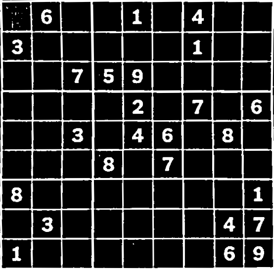
Here is the result of the warping:

warped grid — Warped (straightened) grid

More detail on perspective transformations ⇩

OpenCV comes with a function called getPerspectiveTransform. I had to write the Julia version of this myself. To explain it properly, I would need to explain pinhole cameras, projection matrices, rotation matrices and more. Here is a source which does that: estimating a homography matrix. For now, all I am going to say is that the calculations reduce to multiplication of every pixel with a special matrix called a homography matrix: $$ \begin{bmatrix} u' \\ v' \\ w \\ \end{bmatrix} = \begin{bmatrix} c_{11} & c_{12} & c_{13} \\ c_{21} & c_{22} & c_{23}\\ c_{31} & c_{32} & 1 \\ \end{bmatrix} \begin{bmatrix} x \\ y \\ 1 \\ \end{bmatrix} $$ We then calculate the warped points as: $$ u = \frac{u'}{w} = \frac{c_{11}x+c_{12}y+c_{13}}{c_{31}x+c_{32}y + 1}, \; v = \frac{v'}{w} = \frac{c_{21}x+c_{22}y+c_{23}}{c_{31}x+c_{32}y + 1} $$ We have 8 unknowns in $c_{ij}$ and 8 equations from 4 pairs of $(x, y)$ to $(u, v)$. We can rearrange these 8 equations into a single linear algebra problem: $$ \begin{bmatrix} u_1 \\ u_2 \\ u_3 \\ u_4 \\ v_1 \\ v_2 \\ v_3 \\ v_4 \end{bmatrix} = \begin{bmatrix} x_1 & y_1 & 1 & 0 & 0 & 0 & -x_1u_1 & -y_1u_1\\ x_2 & y_2 & 1 & 0 & 0 & 0 & -x_2u_2 & -y_2u_2\\ x_3 & y_3 & 1 & 0 & 0 & 0 & -x_3u_3 & -y_3u_3\\ x_4 & y_4 & 1 & 0 & 0 & 0 & -x_4u_4 & -y_4u_4\\ 0 & 0 & 0 & x_1 & y_1 & 1 & -x_1v_1 & -y_1v_1\\ 0 & 0 & 0 & x_2 & y_2 & 1 & -x_2v_2 & -y_2v_2\\ 0 & 0 & 0 & x_3 & y_3 & 1 & -x_3v_3 & -y_3v_3\\ 0 & 0 & 0 & x_4 & y_4 & 1 & -x_4u_4 & -y_4v_4 \end{bmatrix} \begin{bmatrix} c_{11} \\ c_{12} \\ c_{13} \\ c_{21} \\ c_{22} \\ c_{23} \\ c_{31} \\ c_{32} \end{bmatrix} $$ Here is the code:

function get_perspective_matrix(source::AbstractArray, destination::AbstractArray)
    if (length(source) != length(destination))
        error("$(length(source))!=$(length(destination)). Source must have the same number of points as destination")
    elseif length(source) < 4
        error("length(source)=$(length(source)). Require at least 4 points")
    end
    indx, indy = 1, 2
    n = length(source)
    A = zeros(2n, 8)
    B = zeros(2n)
    for i in 1:n
        A[i, 1] = source[i][indx]
        A[i, 2] = source[i][indy]
        A[i, 3] = 1
        A[i, 7] = -source[i][indx] * destination[i][indx]
        A[i, 8] = -source[i][indy] * destination[i][indx]
        B[i] = destination[i][indx]
    end
    for i in 1:n
        A[i + n, 4] = source[i][indx]
        A[i + n, 5] = source[i][indy]
        A[i + n, 6] = 1
        A[i + n, 7] = -source[i][indx] * destination[i][indy]
        A[i + n, 8] = -source[i][indy] * destination[i][indy]
        B[i + n] = destination[i][indy]
    end
    M = inv(A) * B # M is a vector
    M = [
        M[1] M[2] M[3];
        M[4] M[5] M[6]'
        M[7] M[8] 1
    ] # M is back to being a matrix
    M
end

Now that we have our matrix, we have a problem: our matrix won't map a set of discrete pixels to another set of discrete pixels. Thankfully the package ImageTransformations.jl handles this for us. It uses the backwards algorithm: instead of warping our pixels to the rectangle, it warps pixels back from the rectangle to the quadrilateral and then interpolates a colour from the nearby pixels it lands in. This is why the perspective_transform function uses the inverse matrix invM.

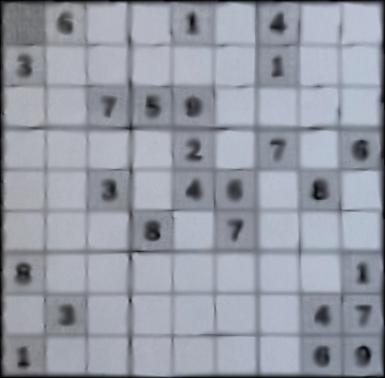
We can see the effect of the linear interpolation by performing multiple warps. This is what the image looks like after warping to and back 50 times:

If we change perspective in reality, we gain information. But by virtually changing perspective we lose information. For a single warp however this loss in information is small and not serious.

Digit detection and extraction

Now that the grid is a rectangle we can divide it into 9×9 cells - regions of interest - and check whether a digit is present in each cell. I’ve added some padding so that there is overlap between each cells. This provides a margin of error for the straightening. I’ve separated the check for a digit into two questions:

Is there a component in the centre of the region of interest?
If yes, what are the bounds and centre of this component?

Answering the second questions allows us to extract the digit which we can then send off to our machine learning algorithm. That is explained in the next section. For now, here is the digit extraction loop in full:

GRID_SIZE = (9, 9)
function extract_digits_from_grid(
    image::AbstractArray,
    predictor; 
    offset_ratio::Float64=0.1,
    detect_options...
    )
    height, width = size(image)
    step_i = ceil(Int, height / GRID_SIZE[1])
    step_j = ceil(Int, width / GRID_SIZE[2])
    offset_i = round(Int, offset_ratio * step_i)
    offset_j = round(Int, offset_ratio * step_j)

    grid = zeros(Int, GRID_SIZE)
    centres =  [(-1.0, -1.0) for i in 1:GRID_SIZE[1], j in 1:GRID_SIZE[2]]
    confidences = zeros(Float32, GRID_SIZE)

    for (i_grid, i_img) in enumerate(1:step_i:height)
        for (j_grid, j_img) in enumerate(1:step_j:width)
            prev_i = max(1, i_img - offset_i)
            prev_j = max(1, j_img - offset_j)
            next_i = min(i_img + step_i + offset_i, height)
            next_j = min(j_img + step_j + offset_j, width)
            RoI = image[prev_i:next_i, prev_j:next_j]
            if detect_in_centre(RoI; detect_options...)
                digit, centre = extract_digit(RoI; detect_options...)
                label, confidence = predictor(digit)
                grid[i_grid, j_grid] = label
                confidences[i_grid, j_grid] = confidence
            else
                centre = (step_i/2, step_j/2)
            end
            centres[i_grid, j_grid] = (centre[1] + prev_i, centre[2] + prev_j)
        end
    end
    grid, centres, confidences
end

The next two sections detail the centre component detection and bounding box algorithms. The predictor is detailed in part 5.

Centre component detection

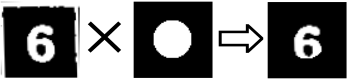
Here is a simple algorithm to detect whether or not there is a component in the centre:

Draw a white circle in the middle of a blank image the same size as the region of interest.
Element-wise multiply the circle kernel with the region of interest.
If the ratio of non-zero pixels to the circle area is greater than some threshold return true, else false.

This is what it looks like:

Here is the code:

function detect_in_centre(image::AbstractArray; 
    radius_ratio::Float64=0.25, threshold::Float64=0.10
    )
    height, width = size(image)
    radius = min(height, width) * radius_ratio
    kernel = make_circle_kernel(height, width, radius)
    conv = kernel .* image
    detected = sum(conv .!= 0)/(pi * radius * radius) > threshold
    detected
end

The ratio for the digits lies between 15%-50% so I’ve set the threshold at a conservative 10%. The assumption is that the machine learning model will be able to distinguish between random artifacts and true digits; we’re just removing the most obviously empty cells.

Lastly, here is code to make a circle with discrete pixels:

function make_circle_kernel(height::Int, width::Int, radius::Float64)
    kernel = zeros((height, width))
    centre = (width/2, height/2)
    for i in 1:height
        for j in 1: width
            z = radius^2 - (j - centre[1])^2 - (i - centre[2])^2
            if z > 0
                kernel[CartesianIndex(i, j)] = 1
            end
        end
    end
    kernel
end

Component extraction

Once we are sure the region of interest is not empty, we can extract the digit. We could use the same contour algorithm as in part 2. However we want all the digit’s pixels not just the border. A better approach is the concept of connected components, where each connected component is made up of non-zero pixels that are neighbours of each other. The simplest of these algorithms is a floodfill approach: find one pixel, then determine its neighbours and those neighbours’ neighbours and so on. I’ve used a more complex and efficient algorithm provided by ImageMorphology.jl called label_components. I must confess, I don’t fully understand it. You may inspect the source code here. This function returns a matrix where each component’s pixels have a unique index, starting from 1. For example, here is a label map for the whole image:

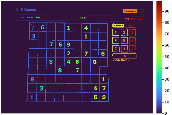
connected components — Source code: `heatmap(labels, yflip=true, c=:turbo, border=:none)`

Doing this for each small region of interest allows us to extract the digits with a tight bounding box while removing all other components. Here is the full code:¹

function extract_digit(image_in::AbstractArray; detect_options...)
    image = copy(image_in)
    # have to binarize again because of warping
    image = binarize(image, Otsu()) # global binarization algorithm
    # check each unique connected component in the image
    labels = label_components(image) 
    for i in 1:length(unique(labels))
        image_label = copy(image)
        image_label[labels .!= i] .= 0
        if detect_in_centre(image_label; detect_options...)
            return extract_component_in_square(image_label)
        end
    end
    height, width = size(image)
    image, (height/2, width/2)
end

function extract_component_in_square(image_label::AbstractArray)
    stats = calc_connected_component_statistics(image_label .> 0, 1)
    width_label = abs(stats.right - stats.left)
    height_label = abs(stats.bottom - stats.top)
    length_  = max(width_label, height_label)

    # note: the centroid is not a good choice for a visual centre
    centre = (stats.top + Int(round(height_label/2)), stats.left + Int(round(width_label/2)))

    # make square
    height, width = size(image_label)
    top = max(1, floor(Int, centre[1] - length_/2))
    left = max(1, floor(Int,centre[2] - length_/2))
    bottom = min(height, ceil(Int, centre[1] + length_/2))
    right = min(width, ceil(Int, centre[2] + length_/2))
    image_label[top:bottom, left:right], centre
end

This function uses a struct which stores information about each connected component:

struct ConnectedComponentStatistics
    left::Int
    top::Int
    right::Int
    bottom::Int
    area::Int
    centroid::Tuple{Float64, Float64}
end

It is calculated from a labels matrix as follows:

function calc_connected_component_statistics(labels::AbstractArray, label::Int)
    height, width = size(labels)

    left = width
    top = height
    right = 0
    bottom = 0
    area = 0
    Cx, Cy = 0.0, 0.0

    for i in 1:height
        for j in 1:width
            if labels[i,j] == label
                area += 1
                left = min(left, j)
                top = min(top, i)
                right = max(right, j)
                bottom = max(bottom, i)
                Cx += 1.0
                Cy += 1.0
            end
        end
    end
    ConnectedComponentStatistics(left, top, right, bottom, area, (Cx/area, Cy/area))
end

Next section

Now that we have individual digits we can pass them to our machine learning function. This is explained next in part 4.

We need to binarize again to remove distortions from warping. Originally I used the AdaptiveThreshold method which applies different thresholds through out the image. This is needed for a large complex image. Here we have much smaller images so a more straightforward algorithm called Otsu’s method can be used. This automatically calculates and applies a single threshold for the whole image. This threshold minimises the intra-class variance - it attempts to set a threshold such that all the pixels within each class (background and foreground) have the most similar values possible. ↩

← Previous Post Next Post →