Wrapping up the Sudoku OCR reader series.
Update 5 August 2023: code refactoring.
This post is part of a series. The other articles are:
All code is available online at my repository: github.com/LiorSinai/SudokuReader-Julia.
Part 5
Thank you for following along until now. This final part is split into the following sections:
Integrating code
First the required imports:
using Images
using Plots
using Flux
using BSON

include("GridDetection/GridDetection.jl")
using .GridDetection
using .GridDetection.PerspectiveTransformations
include("DigitDetection/DigitExtraction.jl")
using .DigitExtraction
Now that we have all the pieces assembled, we can pass the outputs from one part as the input to the next:
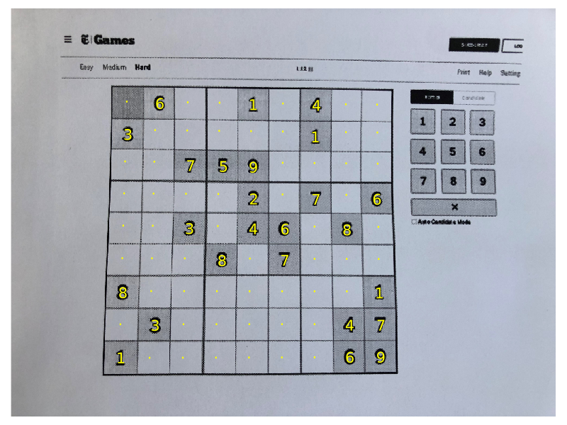
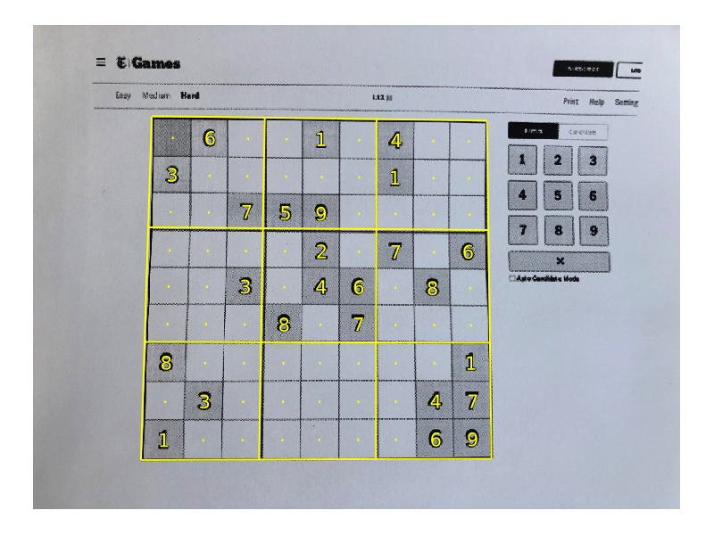
image_path = "images/nytimes_20210807.jpg";
image = load(image_path)

blackwhite, quad = detect_grid(
    image;
    max_size=1024,
    blur_window_size=5, σ=1.1,
    threshold_window_size=15, threshold_percentage=7);
warped, invM = four_point_transform(blackwhite, quad)

grid, centres, confidences = extract_digits_from_grid(
    warped, predictor;
    offset_ratio=0.1,
    radius_ratio=0.25,
    threshold=0.1
    );
The extract_digits_from_grid function requires a predictor which returns a tuple of (label, confidence) for each extracted digit image. Here is one constructed by closing it over the model:
BSON.@load "DigitDetection\\outputs\\LeNet5\\LeNet5_both_e20.bson" model

function predictor(digit_image::AbstractArray)
    logits = digit_image |> prepare_digit_for_model |> model
    idx = argmax(logits)
    probabilities = softmax(logits)
    idx[1] - 1, probabilities[idx]
end

MODEL_SIZE = (28, 28)

function prepare_digit_for_model(digit::AbstractArray; pad_ratio=0.15)
    x = digit
    x = Float32.(x)
    x = pad_image(x; pad_ratio=pad_ratio)
    x = imresize(x, MODEL_SIZE)
    x = reshape(x, MODEL_SIZE[1], MODEL_SIZE[2], 1, 1)
    x
end

function pad_image(image::AbstractArray{T}; pad_ratio=0.15) where T
    height, width = size(image)
    pad = floor(Int, pad_ratio * max(height, width))
    imnew = zeros(T, (height + 2pad, width + 2pad))
    imnew[(pad + 1):(pad + height), (pad + 1):(pad + width)] = image
    imnew
end
Presenting the result
The output of extract_digits_from_grid is three 9×9 matrices: grid, centres and confidences.
The grid has the labels, the centres has the co-ordinates of the centres of the bounding boxes in the warped image, and the confidences the probability of the estimated labels. The latter are zero if no prediction was made.
Drawing text over the original numbers is easy if we use Plots.jl. We will need the perspective_transform function from part 3 to unwarp the centres back to their positions in the original image.
pred_threshold = 0.90
image_out = imresize(image, size(blackwhite));
canvas = plot(image_out, ticks=nothing, border=:none, size=(800, 600));
for i in 1:9
    for j in 1:9
        centre = centres[i, j]
        centre_unwarped = perspective_transform(invM)(centre)
        label =  (probs[i, j] > pred_threshold) ? string(grid[i, j]) : "·"
        annotate!(canvas, centre_unwarped[2], centre_unwarped[1], label, :yellow)
    end
end
Here is the result:
There are two things we can do which greatly improve the presentation:
- Project the grid back on to the original image.
- Align the points which don’t have a prediction.
First a very basic function for making lines which form a grid:
function construct_grid(height::Int, width::Int; nblocks::Int=3)
    grid = []
    step_i = height/nblocks
    step_j = width/nblocks
    for i in 0:nblocks
        push!(grid, [(step_i * i, 1), (step_i * i, width)])
    end
    for j in 0:nblocks
        push!(grid, [(1, step_j * j), (height, step_j * j)])
    end
    grid
end
Then here is a loop for projecting those lines onto the original image:
for line in construct_grid(size(warped, 1), size(warped, 2))
    line_unwarped = map(point -> perspective_transform(invM)(point), line)
    xs = [point[2] for point in line_unwarped]
    ys = [point[1] for point in line_unwarped]
    plot!(canvas, xs, ys, label="", linewidth=2, color=:yellow)
end
Next the align_centres function. We can use the mean of the co-ordinates of the numbers above and below a point to get its $x$ value, and similarly for numbers to the left and right of it for the $y$ value:
function align_centres(centres::Matrix, guides::BitMatrix)
    centres_aligned = copy(centres)
    if size(centres) != size(guides)
         throw("$(size(centres)) != $(size(guides)), sizes of centres and guides must be the same.")
    end
    for i in 1:size(centres, 1)
        for j in 1:size(centres, 2)
            if !guides[i, j]
                # y is common to row i
                if any(guides[i, :])
                    ys = [point[1] for point in centres[i, :]] .* guides[i, :]
                    Cy = sum(ys) / count(guides[i, :])
                else
                    Cy = centres[i, j][1]
                end
                #  x is common to column j
                if any(guides[:, j])
                    xs = [point[2] for point in centres[:, j]] .* guides[:, j]
                    Cx = sum(xs) / count(guides[:, j])
                else
                    Cx = centres[i, j][2]
                end
                centres_aligned[i, j] = (Cy, Cx)
            end
        end
    end
    centres_aligned
end
Applying these two functions makes the result look much more professional:
The final step is to pass the grid into a Sudoku solver, get those numbers back, and project them on to the grid. But I’ll stop here 🙂.
Reflection
This application used several algorithms, some rather complex, to do a task that humans consider trivial. This is not to downplay the effort. The task is a complex one, and we only consider it trivial because our brains have exquisitely adapted to it.
We’ve used several algorithms along the way. It is worth taking stock of all of them and all the parameters that are needed. Some of these parameters are fixed, whether set explicitly or implied. For example, the blurring the same in the horizontal and vertical directions so one parameter is fixed. Others are free and may require hand tuning. Here is a table with an overview of all fixed and free parameters:1
| Step | Algorithm | Fixed parameters | Free parameters |
|---|---|---|---|
| preprocess | imresize | 0 | 1 |
| Gaussian Blur | 2 | 2 | |
| AdaptiveThreshold | 1 | 2 | |
| detect grid | find_contours | 0 | 0 |
| fit_rectangle | 0 | 0 | |
| fit_quad | 0 | 0 | |
| extract digits | four_point_transform | 8 | 0 |
| extract_digits_from_grid | 1 | 1 | |
| detect_in_centre | 0 | 2 | |
| label_components | 0 | 0 | |
| extract_component_in_square | 0 | 0 | |
| predictor | pad_image | 1 | 1 |
| model (LeNet5) | 16 | 44426 | |
| threshold | 0 | 1 |
For the image processing algorithms there are 9 free parameters. Some are subsets of more diverse algorithms. Others are more bespoke and are optimised specifically for one use case.
For machine learning, there are 44,426 free parameters. Compared to the hand crafted image processing algorithms, it is more general and can be repurposed (retrained) for other tasks such as recognising alphabet letters.
As with everything, one does not need to understand these algorithms in depth. But you do need sufficient knowledge of each in order to be able to integrate and fine tune them.
Conclusion
I hope you enjoyed this series and have a working Sudoku OCR reader yourself now.
-
The 16 fixed parameters for LeNet5 are: $k_1$, $k_2$, $s$, $p$, $n_{out}$ for each convolution layer (5×2); $k_1$, $k_2$ for each max pool layer (2×2) and $n_{out}$ for the hidden dense layers (2×1). This count excludes other hyper-parameters such as training parameters, number of layers, number of choices for activation function etc. ↩