Extracting the grid for the Sudoku OCR reader.
Update 5 August 2023: code refactoring.
This post is part of a series. The other articles are:
All code is available online at my repository: github.com/LiorSinai/SudokuReader-Julia.
Part 2 - grid extraction
Table of Contents
Overall process
The main goal here is to find contours in the image. The largest contour is then assumed to be the grid. A “contour” is a line which defines a boundary between the “background” and an “object”. This assumption works well for images where the Sudoku grid dominates the image.1 I found more complicated techniques - e.g. line detections with Hough Transformations - to only add complexity without providing much benefit.
Machine learning could also be used for this problem. For example, MathWorks trained a model to segment an area around the grid. It only trains on 100 images so I do not know how well it generalises. A more general model usually requires a much larger dataset. That could be time consuming to make.
After the largest contour has been found, a quadrilateral is fit to the contour, and that is returned as the grid.
Working with images in Julia
The main package used in this code is JuliaImages.jl.
An image in Julia is an $h\times w$ matrix, where $h$ is the height and $w$ is the width. Its most general type is an AbstractArray.
Each element of the array is a pixel, which can be a native type such as Int or Float64, or a Colorant type such as Gray (1 channel), RGB (3 channels) or RGBA (4 channels).
At the time of publication, JuliaImages.jl defines 18 Color subtypes and 36 TransparentColor subtypes.
This format is convenient because an image can always be expected to be 2D and extra dimensions are handled by the pixel type.
Machine learning often uses an $h\times w \times c$ format, where $c$ is the number of channels.
The function channelview can convert it to a $c \times h\times w$ array, and then permutedims can convert it to a $h\times w \times c$ array:
image_CHW = channelview(img_rgb)
image_HWC = permutedims(img_CHW, (2, 3, 1))
For grayscale images, calling Float64.(image) converts the image directly to a Float64 array.
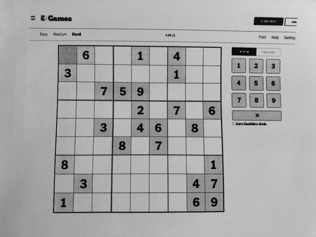
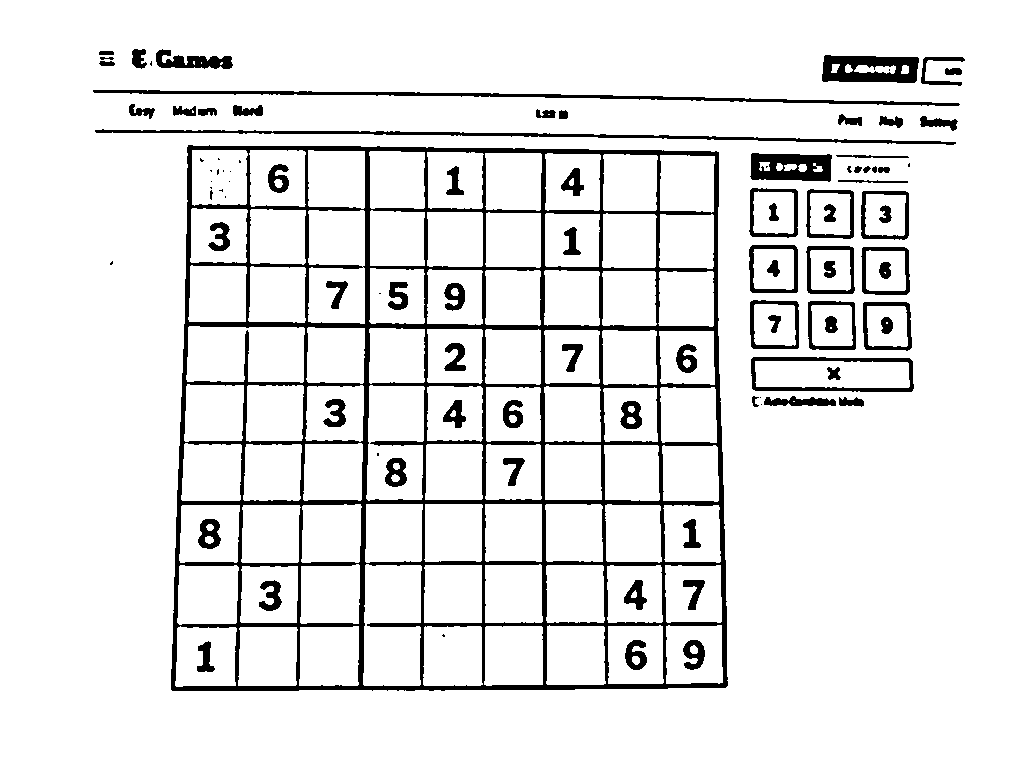
With this knowledge in mind, we can start by loading our image.
using Images

image_path = "images/nytimes_20210807.jpg"
image = load(image_path)
Preprocessing
Resizing
Resizing the image is useful because:
- This speeds up all other operations. Most of them are $O(p)$ where $p=hw$ is the number of pixels. Reducing an image size by 2 in both dimensions reduces the number of pixels by 4, which speeds up operations by the same factor.
- The blurring and adaptive threshold methods that will be described next are not scale invariant. Having a maximum size is insurance that the parameters we pick will always be appropriate.
I found a maximum dimension size of 1024 pixels to be sufficient. We can use it to calculate a ratio and pass this number to our imresize:
ratio = max_size/size(gray, argmax(size(gray)))
if ratio < 1
    gray = imresize(gray, ratio=ratio)
end
Binarize
The next step is to convert the image to black and white. This is because it simplifies the calculations greatly for classic image processing techniques. This is in contrast to machine learning which can easily handle multiple colour channels and where more information is encouraged.
First convert the image to grayscale. This is done by calling Gray.(image). Out of interest, the underlying code from Colors.jl is :
cnvt(::Type{G}, x::AbstractRGB) where {G<:AbstractGray} =
    G(0.299f0*red(x) + 0.587f0*green(x) + 0.114f0*blue(x))
This is a standard grayscale conversion where the green spectrum is more heavily weighted because of a natural bias towards green in human eyes. More information here: www.tutorialspoint.com/dip/grayscale_to_rgb_conversion.htm.
All the pixels now have a value between 0 and 1. Next we need to threshold values so that the values are either 0 or 1.
We could apply a single threshold over the whole picture e.g. blackwhite = gray .< 0.8.
A better method is the adaptive thresholding technique provided by the ImageBinarization.jl package.
This does an intelligent local thresholding.
From the documentation:
If the value of a pixel is $t$ percent less than the average of an $s×s$ window of pixels centered around the pixel, then the pixel is set to black, otherwise it is set to white.
The code is as follows:
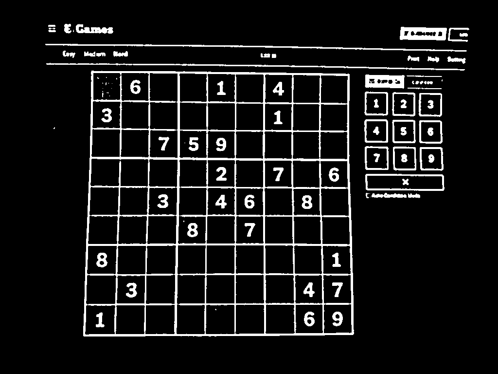
using ImageBinarization

blackwhite = binarize(gray, AdaptiveThreshold(window_size=15, percentage=7))
And the result:
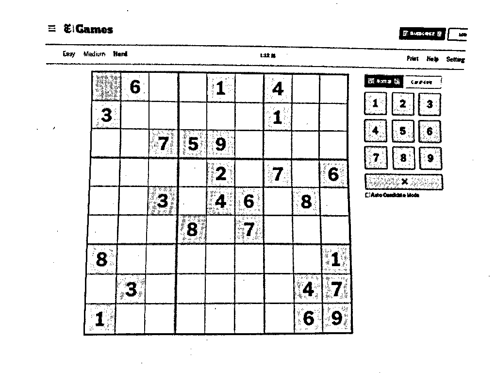
This is what we wanted but there are two problems. Firstly there is a lot of noise - it would be better if we could remove all those small patches. Secondly, for the contour detection we need the contours to be white (have a value of 1) and the background to be black (have a value of 0).
To reduce noise, we can apply an image filter with a Gaussian Kernel from ImageFiltering.jl. After this, every pixel will be a weighted sum of it and its neighbours based on a kernel we give it. The net effect is a blurring of the image.
Here is the code to do this:
using ImageFiltering

window_size = 5
σ = 1
kernel = Kernel.gaussian((σ, σ), (window_size, window_size))
gray = imfilter(gray, kernel)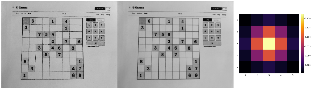
As can be seen in the image, the blurring effect is slight. Of course if we changed the parameters, say σ = 5 and
window_size=21, the effects could be more dramatic:
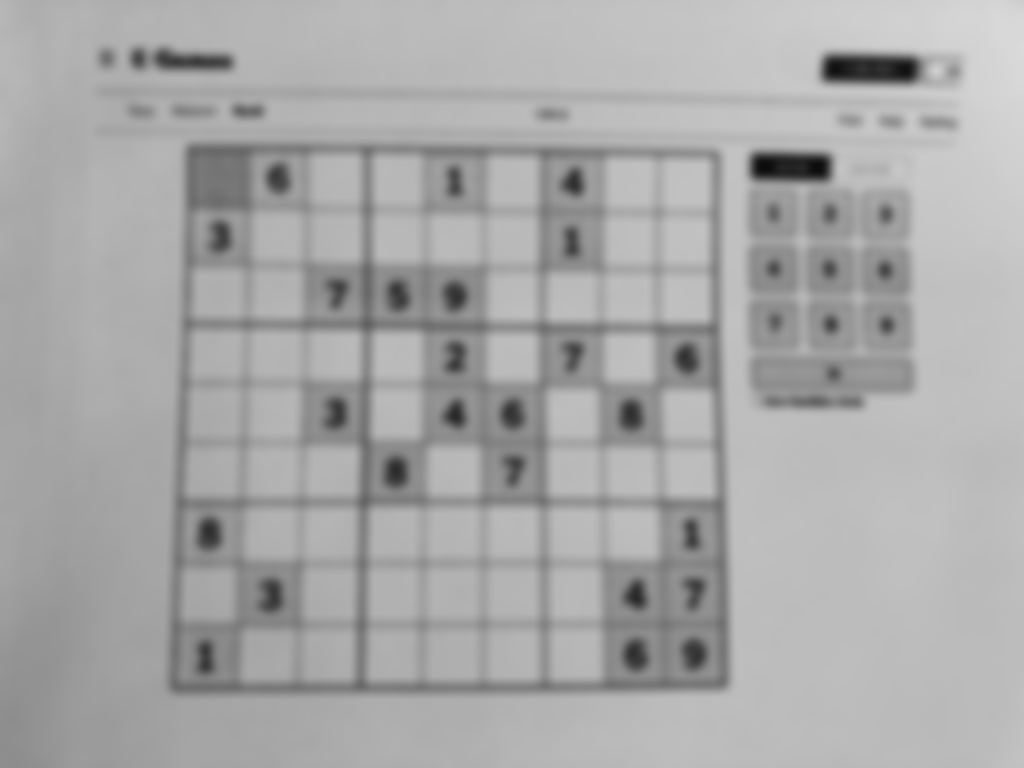
The slight blurring however does have a big effect on the thresholding:
Inverting the image is rather simple. In Julia for loops are fast:
function invert_image(image)
    image_inv = Gray.(image)
    height, width = size(image)
    for i in 1:height
        for j in 1:width
            image_inv[i, j] = 1 - image_inv[i, j]
        end
    end
    return image_inv
end
The result:
Contour Detection
We can finally start looking for contours. The de facto algorithm for doing this is highly specialised, so I will not go into more detail here. For more information please see the 1987 paper by Suzuki and Abe.
I couldn’t find a package with this algorithm (a common occurrence for a young language like Julia).
However thankfully the people at JuliaImages.jl wrote a Julia port of it: contour_detection.
I copied this code and modified it slightly to (1) better follow Julia Conventions and (2) have the option to only return external contours. The code is available here: ImageContours.jl. Please note: this is work in progress. Also I am very proud of the point_in_polygon function, which uses a very robust method from a fairly recent paper.
Here is the result of calling find_contours(blackwhite):
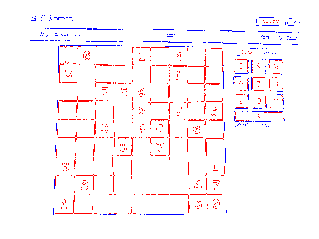
Now we’re getting somewhere! The grid is clearly the largest contour in the image, which we’re going to assume is the general case. With the area_contour function that I also provide, it takes three lines to extract it:
contours = find_contours(blackwhite, external_only=true)
idx_max = argmax(map(area_contour, contours))
contour _max = contours[idx_max]
Quadrilateral fitting
The contour we have is comprised of many points (in this case, 2163). We want to simplify it to a 4 point quadrilateral. There are few ways to do this. I found the easiest was to first fit a rectangle to the contour. Its corners can be found as the min and max of the $x$ and $y$ values of the contour points. Then fit a quadrilateral by finding the points on the contour that minimise the rectangular distance to each corner. In a single equation:
\[min(|x_i - r_{x,j}| + |y_i - r_{y,j}|) \; \forall \; i \in c, \; j \in \{1, 2, 3, 4 \}\]Where $r$ is the rectangle and $c$ is the contour.
Here is the code:
function fit_rectangle(points::AbstractVector)
    # return corners in top-left, top-right, bottom-right, bottom-left
    min_x, max_x, min_y, max_y = typemax(Int), typemin(Int), typemax(Int), typemin(Int)
    for point in points
        min_x = min(min_x, point[1])
        max_x = max(max_x, point[1])
        min_y = min(min_y, point[2])
        max_y = max(max_y, point[2])
    end

    corners = [
        CartesianIndex(min_x, min_y),
        CartesianIndex(max_x, min_y),
        CartesianIndex(max_x, max_y),
        CartesianIndex(min_x, max_y),
    ]

    return corners
end

function fit_quad(points::AbstractVector)
    rect = fit_rectangle(points)

    corners = copy(rect)
    distances = [Inf, Inf, Inf, Inf]

    for point in points
        for i in 1:4
            d = abs(point[1] - rect[i][1]) + abs(point[2] - rect[i][2])
            if d < distances[i]
                corners[i] = point
                distances[i] = d
            end
        end
    end
    return corners
end
Finally, the result, which we can return as our grid:
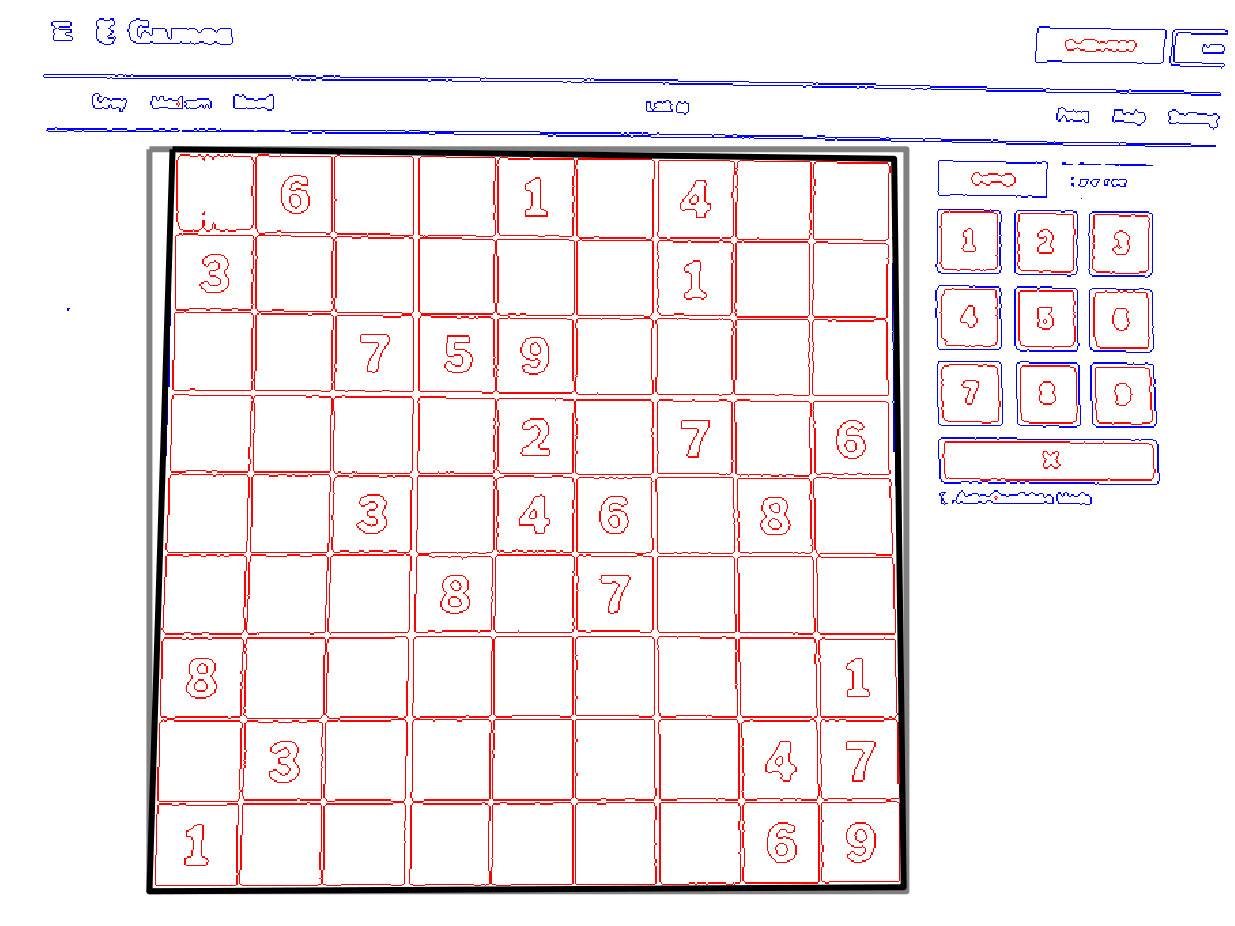
Next section
Now that we have the grid, we can extract the digits inside it. This is explained next at part 3.
-
More robust methods could check for the “squareness” of the contour. For example, $\frac{l_{max}}{l_{min}} - 1 < \epsilon $ where $l$ is the length of a side and $\epsilon$ is some small number. ↩