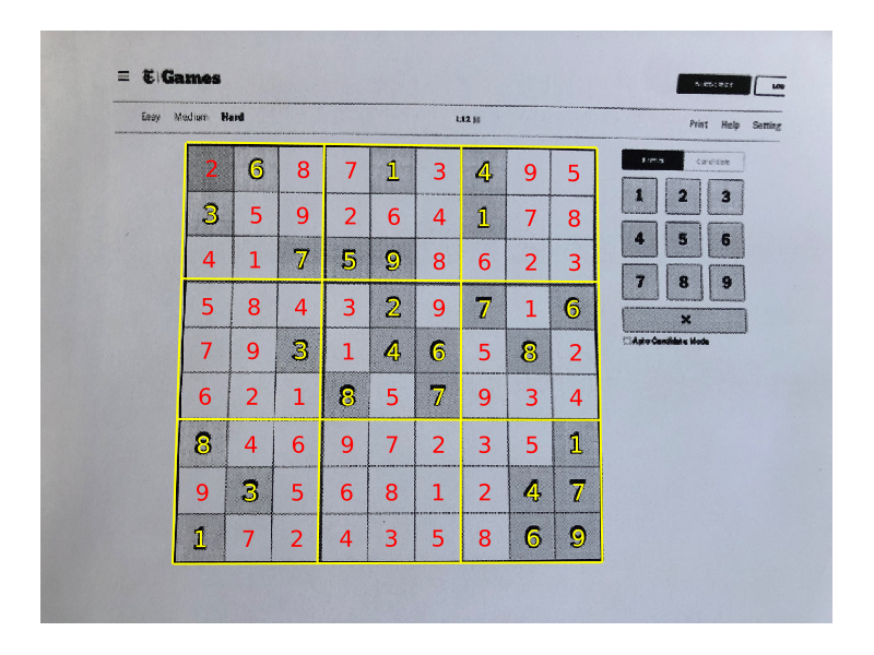
A Sudoku OCR reader written in Julia.
This is part of a series. The other articles are:
All code is available online at my repository: github.com/LiorSinai/SudokuReader-Julia.
Introduction
My sudoku solver post from a year ago remains the most popular post on this website by a wide margin. That post describes the levels of Sudoku difficulty and details an algorithm that can solve all of them. It then implements one in Python. It is quite neat if I do say so myself. It can solve any Sudoku puzzle in under a second (if it is solvable).
I had already seen people take this concept one step further, such as Raghav Virmani’s awesome LinkedIn post on an optical character recognition (OCR) reader and solver. In his post he places a print-out of a Sudoku puzzle in front of his camera, solves it in real time and projects the solution back on to the grid. Naturally I thought this was awesome and implemented it myself in Python. I did not write a blog post on it because there are many great blog posts already: see PyImageSearch’s article or the series of articles at AI Shack.
Then 2 weeks back it was the Julia conference which I really enjoyed. I am a big fan of Julia. While I still like Python, I much prefer Julia. I find it to be a much more robust, stable and clean programming language. So I decided to implement an OCR reader for Sudoku in this new, growing programming language. This post details my journey. To the best of my knowledge, there are no other articles detailing this in Julia at this moment in time.
Pipeline
I followed the same algorithm as the original C++ and Python tutorials. It uses classic image processing techniques to extract the grid and then the digits, and then it uses machine learning to classify the digits.
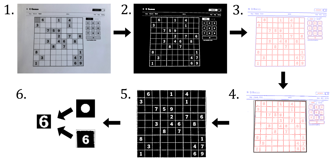
The algorithm is as follows:
- Input an image.
- Preprocess the image by:
- Blurring it slightly with a Gaussian kernel to remove noise.
- Transform to binary (0 or 1) using adaptive thresholding.
- Detect contours using the border following technique of Suzuki and Abe.
- Assume the largest contour is the grid. Fit a quadrilateral to this grid.
- Straighten the region in the quadrilateral to a rectangle. This is done with a homography transformation matrix.
- Divide the rectangle into 9×9 grid. For each cell:
- Detect if there is an object in the centre. This is done by finding the product of the cell with a circle kernel.
- If there is an object, extract the first large connected component in the centre as the digit.
- Pass the digit to a machine learning network and receive a prediction back. If the softmax probability is above a threshold, accept the prediction, else reject it.
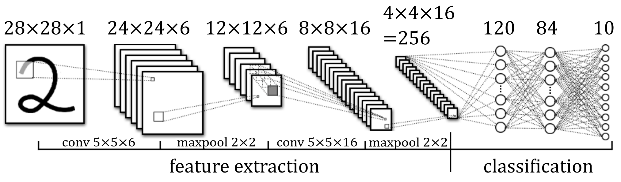
The machine learning algorithm should not be seen as a black box. It uses LeNet5 and is trained on the Char74K dataset. Importantly, it is not trained on the popular MNIST dataset and it does not use newer architectures. I explain my reasons for this and the difficulties I had in part 4.
You could perhaps use machine learning for more parts of the pipeline. See for examples MathWorks’ posts. Personally I think machine learning can be tricky to implement and expensive to train, and should only be reserved for the hardest task. That is, digit classification.
The algorithm is not robust and is prone to false positives. That is, because of the weak assumptions made, anything vaguely representing a grid - a painting or a cupboard - will be identified as the Sudoku grid. The machine learning algorithm is also not robust to noise so it will then “see” numbers in this random object. It is up to the user to avoid these problems by only feeding in clear, well lit images of Sudoku grids.
For an in-depth explanation of each step, please see the following posts:
- Preprocessing, grid extraction and quadrilateral fitting: part 2.
- Image warping and digit extraction: part 3.
- Digit classification using machine learning: part 4.
- Demonstration of the full pipeline and conclusion: part 5.
Comparison with Python
Having done it first in Python gave me perspective. Firstly, I think Python is a better choice for this task. That is a negative way to start off a series that is supposed to promote Julia. But Julia does have an infamous “first time to plot” problem, and this task is mostly about plotting and processing single images. Julia imposes an upfront cost of an initial slow compile time for enhanced performance afterwards. It can take 2 and a half minutes to run the code base from start to finish the first time. After that it takes a few seconds but that’s already too late. Meanwhile in Python it takes a few seconds to run through the whole pipeline every time. That said, I still think this application is worthwhile as a learning exercise.
The machine learning is where Julia really shined. Julia is built for scientific programming and number crunching. This is what it excels at it. Flux - the main machine learning package - is lightweight, flexible and elegant. I have written code with TensorFlow, PyTorch and MXNet, and I can easily say Flux is the nicest of them all. It is also very fast. Here you recuperate the slow compile times with fast training times - less than 2 minutes to fully train a model through 20 epochs of 10,000 data points each.
A big advantage of the Julia packages is that they are entirely written in Julia.
The Python interpreter is slow so packages tend to be written in Cython, C or C++ for performance reasons.
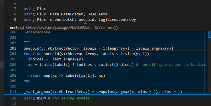
But Julia itself is inherently fast and stable, and so the underlying code is Julia all the way down.
In practice this means you can use the @edit macro in the REPL or right click a piece of code in an IDE and you’ll be able to go straight to the definition. This simply isn’t possible with Python packages that only exist as Python wrappers around the original codebase.
This has several advantages. Firstly it lifts the lid off of functions. Most of OpenCV’s functions were a black box to me, unless I searched the C++ code on GitHub to understand it better.
In Julia, I could jump straight to the image processing functions and back at will.
Secondly you can easily adapt the code. I didn’t like Flux’s original train! function, but it was very easy to copy it and customise it as I liked. Lastly, it allows you to pick up on best practices and advanced techniques used by popular packages. In Python you miss out on all of this.
Speaking of packages, the Julia ecosystem is very different to the Python ecosystem. Life grows under the constraints imposed by the environment, and the constraints imposed by Julia and Python are very different indeed. Python is a dynamic language. This makes it easy to learn but it is not type safe and is prone to runtime errors. Also, as just discussed above, the underlying code is often not written in Python so two languages have to be maintained. The result is massive monolithic packages that are carefully controlled and curated. Meanwhile Julia is also a dynamic language, but it is (mostly) type safe and has strictly controlled modules. This has made all the difference. It’s very easy to share and integrate Julia code. You can use someone else’s package directly with your own and it won’t break. The result is a fragmented ecosystem with many small packages.1
| Python | Julia | |
|---|---|---|
| Image processing |
|
|
| Machine learning |
|
|
| Files |
|
|
| Plotting |
|
|
| Linear Algebra |
|
|
I like to think of the Python ecosystem as buildings carefully designed by architects who know their construction very well, while Julia’s is like a stack of Lego bricks that can be stuck together. As first detailed in the article “The unreasonable effectiveness of the Julia programming language”, Julia has caught like wildfire in academic institutions because of this. This was very evident at the very academically focused Julia Con, with all the many varieties of research code that is now written in Julia. Academia is naturally a collaborative environment unlike the closely guarded intellectual property of industry. It was always going to embrace a coding language that supported this.
Julia is built to be modular. I think it is this single reason, more than Julia’s speed, more than its syntax and design and compiler and metaprogramming and other features, that will ultimately be the reason Julia one day overtakes Python.
One last thing. There is a negative aspect to this sharing: packages don’t always “play nice” so that they can easily integrate with other packages. For example packages should abide by the following etiquette:
- Type safe functions that will throw errors if nonsensical types are passed.
- Extensions where appropriate of useful Base functions such as
zero,firstandsize. - No exports of commonly used words. Base itself is a frequent but tolerated offender. Worse offenders are NNlib.jl which reserves σ for the sigmoid function2 and Images.jl which reserves the ubiquitous keyword data. Thankfully at least sense has prevailed at ImagesMetaData.jl, and
datahas been deprecated in favour ofarraydata. - Minimal restrictions on package requirements or frequent updates to packages. If a package from 2 years ago is going to force my Flux to be stuck 8 versions behind the current version, that package is going to go. (As a user you can mitigate this by creating package environments.)
Next section
The coding tutorial starts next at part 2.
-
Even the popular packages like Images.jl and Flux.jl are mostly composed of smaller packages. This is fundamentally different to the way OpenCV and TensorFlow are composed of smaller parts, because those smaller packages can and are used separately to the main packages. Some packages like Scikit-learn have no equivalent in Julia. I’ve since come to appreciate there never will be. But there will be packages which do one thing from Scikit-learn really well. ↩
-
Wikipedia lists at least 25 uses for the lower case σ letter. ↩