On convolutional neural networks, overly large models and the importance of understanding your data.
Update 5 August 2023: code refactoring and notice on changes in Flux 0.13.9.
This post is part of a series. The other articles are:
All code is available online at my repository: github.com/LiorSinai/SudokuReader-Julia.
Part 4 - machine learning
Table of Contents
A mistaken assumption
When I initially envisioned this blog post, I thought I wouldn’t have much to talk about with regards to machine learning. Digit recognition is the entry level problem of machine learning. It is incorporated into almost every beginner course on the topic. My assumption was you as the reader have done this before and I would only need to present the code. The model would be copied off the first tutorial I found on the internet and would be trained on the MNIST dataset. But I found MNIST ill-suited to the task at hand and the models subpar. In particular:
- The handwritten MNIST dataset resulted in many false positives with computer font digits. This was most pronounced between 1s, 2s and 7s and between 6s and 0s.
- The models were unnecessarily large. I used a 44,000 parameter model to solve this problem. Some other models had over 1 million parameters.
I’ll now delve further into each of these issues.
Data
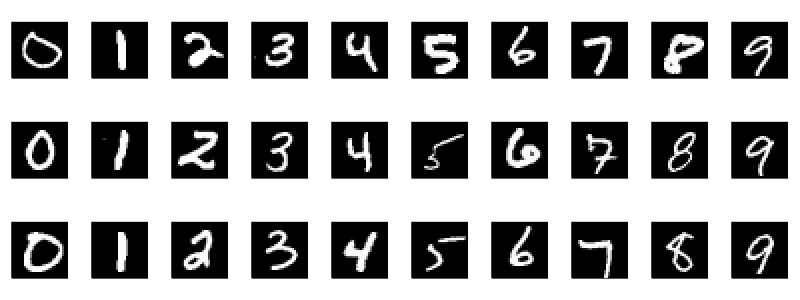
The Modified National Institute of Standards and Technology database (MNIST) is a large set of 70,000 labelled handwritten digits. Here is a sample of the digits:1,2
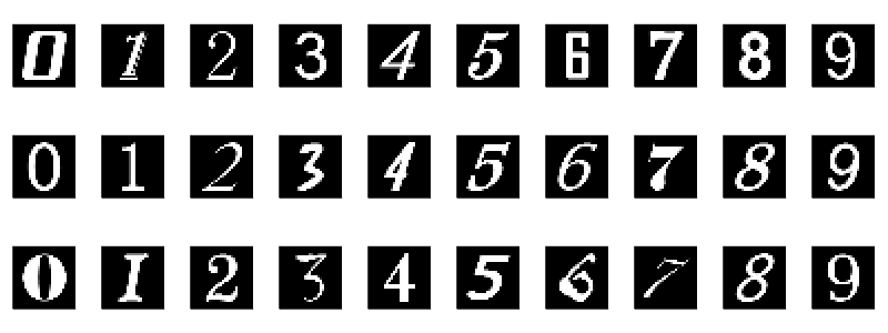
I trained my model and then discovered very quickly that despite a 99% test accuracy, it was not the best dataset for a model that will mostly be aimed at computer printed digits. To understand why, let us look at a different dataset, the Char74K dataset. It is based on computer fonts:
Here is a general comparison of the mean image of each digit for each dataset:
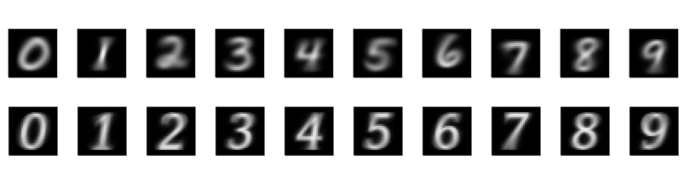
The computer 1s tend to have a hook that handwritten 1s don’t have. The handwritten 4s are open at the top whereas computer 4s are closed. The circle in handwritten 6s tends to be smaller than the circle in computer 6s. All these small differences make a big impact.
As an experiment, I trained the LeNet5 model (detailed below) on the MNIST dataset and evaluated it on the Char74k dataset. While it had a 98.7% test accuracy for MNIST data, this only translated to a 81.3% accuracy on the whole Char74k dataset. So these datasets are strongly correlated but that is not enough for the required task. Here is the confusion matrix for the Char74k dataset:
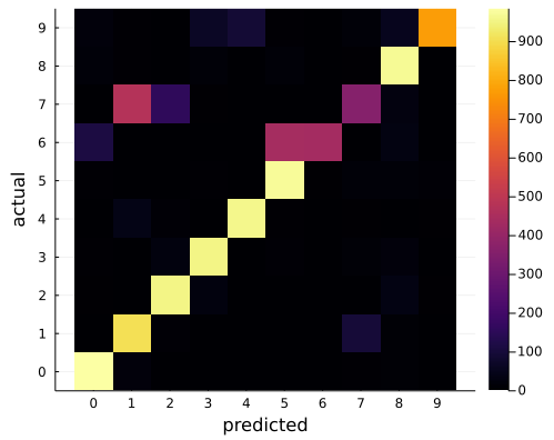
As expected, 7, 1 and 2 are often confused. So was 6s with 5s and - to a less extent - 6s with 0s. This sort of confusion also appeared with the few Sudoku images I tried. Training the model on the Char74k data removed this problem.
Going the other way, a model trained on the Char74k dataset to a 99.1% test accuracy only achieved a 54.1% accuracy on the MNIST data. I found this acceptable because the target is computer fonts not handwritten digits. Its overall performance with the Sudoku images was much better.
Another strategy is to train on both: 10,000 Char74k figures and 10,000 MNIST figures. This model has a test accuracy of 98.1%. For the separate datasets (train &test) it is 99.4% on the Char74k data and 98.8% on the MNIST data. A flaw of this model is that 42 times it confused 2s for 7s. (Out of 4000 2s and 7s that is acceptable.) Otherwise the second largest off-diagonal value in the confusion matrix was 12. Overall, this model seemed to perform slightly worse on the Sudoku images.
Models
I eventually used the LeNet5 model originally published in 1998. Its architecture is as follows:
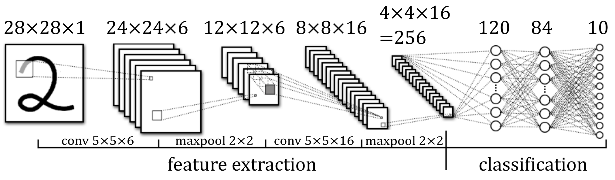
It is a convolutional neural network. If you’re unfamiliar with this type of neural network, please see this article for a guide on how they work.
In Julia code, LeNet5 is built as follows:3
model = Chain(
	Conv((5, 5), 1=>6, relu),
	MaxPool((2, 2)),
	Conv((5, 5), 6=>16, relu),
	MaxPool((2, 2)),
	Flux.flatten,
	Dense(256, 120, relu),
	Dense(120, 84, relu),
	Dense(84, 10),
	)
This was not the first model I encountered. Instead that was a huge 1.2 million parameter model on a blog post. It worked, but it is unnecessarily large and slow. It is built as follows:
model = Chain(
	Conv((3, 3), 1=>32, stride=1, pad=0, relu),
	Conv((3, 3), 32=>64, stride=1, pad=0, relu),
	MaxPool((2, 2)),
	Dropout(0.25),
	Flux.flatten,
	Dense(9216, 128),
	Dropout(0.5),
	Dense(128, 10),
    )
This model is similar to LeNet5 but it has a few key differences. Firstly, it has about 4.3× the number of kernels.
Secondly, it does 2× the amount of convolutions per Conv step (steps of 3 instead of 5).
Lastly it only down samples once with a MaxPool.
Down sampling again by a factor 2 in both directions would have reduced the total pixel size by 4, which in turn reduces
the parameter space by approximately 4. So 225,034 parameters instead of over a million.
I then investigated a few other models. Here is a summary of my findings for models trained only on the Char74k dataset:
| name | train accuracy (%) | test accuracy (%) | inference time (ms) | file size (kB) | parameters | |
|---|---|---|---|---|---|---|
| 1 | cnn_mastery | 99.99 | 98.77 | 0.1547 | 2119.68 | 542230 |
| 2 | LeNet5 | 99.51 | 98.67 | 0.0806 | 183.0 | 44426 |
| 3 | cnn_medium | 99.37 | 98.67 | 0.1355 | 79.4 | 18378 |
| 4 | cnn_huge | 99.26 | 98.13 | 0.8164 | 4689.92 | 1199882 |
| 5 | cnn_small | 98.62 | 97.74 | 0.0576 | 27.7 | 5142 |
| 6 | nn_fc | 98.43 | 96.75 | 0.0023 | 103.0 | 25450 |
Th cnn_huge model comes in 4th place despite its large amount of parameters. It is 10 times slower and 25.6 times larger than LeNet5. You may notice it still only has an inference time of 0.8ms and a file size of 4.6MB. It took 10 minutes to train as opposed to 2 minutes for LeNet5. These numbers are still small, so what is the fuss? I just greatly dislike increasing complexity and reducing performance for no reason.
The fastest model is nn_fc. It only has fully connected layers with no convolutions. Here is its architecture:
model = Chain(
        Flux.flatten,
        Dense(784, 32, sigmoid),
        Dense(32, 10),
    )
This model is prone to errors because it does not take the structure of the image to account. So very weirdly, you can swap rows and columns and not affect the prediction. Clearly this limits the overall accuracy of the model.
LeNet5 is a good balance between slow convolutions with few parameters and large but fast fully connected layers. It reduces the feature space by a factor of 3 from 784 pixels to 256 kernel pixels before classification. I still think it is too large - the smallest model in the table is 1/8th its size. But for 183kB against 28kB, I think it’s a reasonable tradeoff for a 1% increase in accuracy.
Training
I followed the tutorials of Nigel Adams and Clark Fitzgerald. Julia is a young language and is still short on resources and tutorials for Flux. I am therefore glad these two ventured into the unknown early with their articles.
I used the digits from the Char74k dataset, specifically Sample001-Sample010 in EnglishFnt.tgz.
It is useful to convert the Char74k dataset to the MNIST format so the same model can be used for both datasets.
This script will do that (be sure to have the correct inpath for your data):
using Images

inpath = "..\\..\\datasets\\74k_numbers"
outpath = inpath * "_28x28"
include("..\\utilities\\invert_image.jl");

if !isdir(outpath)
    mkdir(outpath)
end

for indir in readdir(inpath)
    println("working in $(joinpath(inpath, indir))")
    outdir = joinpath(outpath, string(parse(Int, indir[(end-1):end]) - 1))
    if !isdir(outdir)
        mkdir(outdir)
    end
    num_saved = 0
    for filename in readdir(joinpath(inpath, indir))
        num_saved += 1
        image = load(joinpath(inpath, indir, filename))
        image = imresize(image, (28, 28))
        image = invert_image(image)
        save(joinpath(outdir, filename), image)
    end
    println("saved $num_saved files to $outdir")
end
Now we can look into the training. Here are all the imports we will need:
using Flux
using Flux: Data.DataLoader
using Flux: onehotbatch, onecold, logitcrossentropy
using BSON
using StatsBase: mean
using Random
using Printf
I also wrote a few helper functions at ml_utils.jl. For example, here is the function to load the data:
function load_digit_images(data_dir::AbstractString)
    # data is images within a folder with name data_dir/label/filename.png
    digits = [0, 1, 2, 3, 4, 5, 6, 7, 8, 9]

    data = Array{Float32, 3}[] # Flux expects Float32 only, else raises a warning
    labels = Int[]
    for digit in digits
        digit_dir = joinpath(data_dir, string(digit))
        println("Loading data from $digit_dir")
        for filename in readdir(digit_dir)
            image = load(joinpath(data_dir, string(digit), filename))
            image = Flux.unsqueeze(Float32.(image), 3)
            push!(data, image)
            push!(labels, digit)
        end
    end
    batch(data), labels
end
An important caveat is that the data should be of type Float32. This does noticeably increase the speed of training the model.
Also, the data needs to be in the form height×width×channels×batch_size.
The functions Flux.unsqueeze and Flux.batch do this transform.
Next split the data into train, validation and test sets.
Here is the split_data function:
function split_data(rng::AbstractRNG, X::Array, y::Vector; test_split::Float64=0.2)
    n = size(X)[end]
    n_train = n - round(Int, test_split * n)
    idxs = collect(1:n)
    randperm!(rng, idxs)
    inds_start = ntuple(Returns(:), ndims(data) - 1)
    X_ = X[inds_start..., idxs]
    y_ = y[idxs]
    x_train = X_[inds_start..., 1:n_train]
    y_train = y_[1:n_train]
    x_test  = X_[inds_start..., n_train+1:end]
    y_test  = y_[n_train+1:end]
    x_train, y_train, x_test, y_test
end
It’s best to fix the seed at an arbitrary number so that the data is always “randomly” sorted the same way. This makes comparisons between training runs consistent.
seed = 227
rng = MersenneTwister(seed)
x_train, y_train, x_test, y_test = split_data(rng, data, labels);
y_train = onehotbatch(y_train, 0:9)
n_valid = floor(Int, 0.8*size(y_test, 2))
val_data = (x_test[:, :, :, 1:n_valid], onehotbatch(y_test[1:n_valid], 0:9))
test_data = (x_test[:, :, :, n_valid+1:end], onehotbatch(y_test[n_valid+1:end], 0:9))
The labels need to be one hot matrices for the loss function.
To prevent using extra space, we can use Flux.DataLoader which lazily batches the data. This means it doesn’t create a copy of the data (unlike split_data) when allocating a batch for a small gradient descent step.
train_loader = Flux.DataLoader((x_train, y_train); batchsize=128, shuffle=true)
val_loader = Flux.DataLoader(val_data; shuffle=false)
test_loader = Flux.DataLoader(test_data; shuffle=false)
Now we can load the LeNet5 model from before:
function LeNet5()
  return Chain(
      Conv((5, 5), 1=>6, relu),
      MaxPool((2, 2)),
      Conv((5, 5), 6=>16, relu),
      MaxPool((2, 2)),
      Flux.flatten,
      Dense(256, 120, relu),
      Dense(120, 84, relu),
      Dense(84, 10),
    )
end
model = LeNet5()Flux assumes you know the input and output sizes for the dense layers. Therefore we need to know the output size of the last convolution layer. This can be calculated with the following formula: $$ \left\lfloor \frac{i+2p-k}{s} \right\rfloor + 1 $$ Where $i$ is the input size, $p$ is the pad, $k$ is the kernel (filter) size and $s$ is the stride length. For a very thorough explanation, please see this paper: A guide to convolution arithmetic for deep learning.
In Julia code:
function calc_output_size(input_size::Int, filter_size::Int, stride::Int=1, pad::Int=0)
	floor(Int, (input_size + 2pad - filter_size)/stride) + 1
endoutput_dim = 28
output_dim = calc_output_size(output_dim, 5, 1, 0) # 24
output_dim = calc_output_size(output_dim, 2, 2, 0) # 12
output_dim = calc_output_size(output_dim, 5, 1, 0) # 8
output_dim = calc_output_size(output_dim, 2, 2, 0) # 4
output_size = prod((output_dim, output_dim, 16)) # 256
We then need to define an accuracy function and a loss function:
accuracy(ŷ, y) = mean(onecold(ŷ, 0:9) .== onecold(y, 0:9))
loss(x::Tuple) = Flux.logitcrossentropy(model(x[1]), x[2])
loss(x, y) = Flux.logitcrossentropy(model(x), y)
opt=ADAM()The Flux.logitcrossentropy calculates the following:
The logits are the direct outputs of the model, which can be any real number. The softmax function $\sigma$ converts them to values between to 0 and 1 which sum to 1. That is, it converts them to a probability distribution. Adam is a well known and stable gradient descent algorithm that works well without much fine tuning.
With these function in place, we can simply call Flux.train!(loss, params(model), train_data, opt) and wait for our model to train. But I wanted more. I wanted to create a history of the change in accuracy during training and return it. I wanted to have a print out each time a batch was completed. I wanted to save after every epoch, where an epoch is one full run through the entire training set.
So I copied the definition for Flux.train! and edited it as follows:
function train!(loss, ps, train_data, opt, acc, valid_data; n_epochs=100)
    history = Dict(
        "train_acc" => Float64[],
        "val_acc" => Float64[],
        )
    for e in 1:n_epochs
        print("$e ")
        ps = Flux.Params(ps)
        for batch_ in train_data
            gs = gradient(ps) do
                loss(batch_...)
            end
            Flux.update!(opt, ps, gs)
            print('.')
        end
        # update history
        update_history!(history, model, train_data.data, val_data.data)
        println("")
        # save model
        save_path = output_path * "_e$e" * ".bson"
        BSON.@save save_path model history
    end
    history
end

function update_history!(history::Dict, model, train_data, val_data)
    result = model(train_data[1])
    train_acc = accuracy(result, train_data[2])
    val_result = model(val_data[1])
    val_acc = accuracy(val_result, val_data[2])
    push!(history["train_acc"], train_acc)
    push!(history["val_acc"], val_acc)
    @printf "train_acc=%.4f%%; " train_acc * 100
    @printf "val_acc=%.4f%%; " val_acc * 100
end

start_time = time_ns()
history = train!(
    loss, params(model), train_data, opt,
    accuracy, valid_data, n_epochs=20
    )
end_time = time_ns() - start_time
println("done training")
@printf "time taken: %.2fs\n" end_time/1e9
Here is an example of the training history for LeNet5 trained on the Char74k dataset:
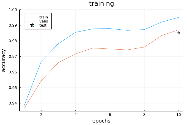
Finally we calculate the final test accuracy on the small test data we had left behind:
test_acc = accuracy(model(test_data[1]), test_data[2])
@printf "test accuracy for %d samples: %.4f\n" size(test_data[2], 2) test_acc
Next section
This was a long section with unexpected detours. I hope you enjoyed it. We can now go to the final section where we can see the results of our model: part_5.
-
In the MNIST data, the 7s and 9sx are lowered with respect to the top of the image and the 6s are slightly raised. I presume this is because when this data was processed the centroid was used as the centre of image. I believe a better choice would have been to use the centre of the bounding box. This is what the digit extraction does in part 3. ↩
-
One can argue that you don’t need to train with zero because there should never be a zero in Sudoku. For the user experience I’d argue it is worth the marginal effort. If the user does have a zero in their image, for whatever reason, it will make the model appear very incompetent if it cannot classify zeros. But this is your personal preference. ↩
-
Flatten is exported by both DataFrames and Flux and therefore needs to be qualified. ↩