Interpolation using quaternions.
This is part of a series. The other articles are:
Table of Contents
Interpolation with Quaternions
Introduction
This is a demo of the two interpolation methods that will be described in this article. Using the default button sets the stick aeroplane to the same settings as the space cruiser in part 1. See the source code here.
In part 1 the problem of finding a satisfying rotation halfway between two other rotations was presented. We now extend this problem statement to any fraction: given an initial rotation at time $t=0$ and a final rotation at $t=1$ find a smooth formula for a rotation at time $t$ where $0 \leq t \leq 1$.
This post will describe two solutions which give slightly different results:
- Lerp: linear interpolation.
- Slerp: spherical linear interpolation.
The equation for lerp is simpler but slerp has a smoother profile. This however is hardly noticeable in above demo.
This post is based on Quaternions, Interpolation and Animation by Erik B. Dam, Martin Koch and Martin Lillholm. Please see this book for more detail on using quaternions in animations and the formulas presented in this post.
Lerp
Because quaternions encode rotations it is possible to linearly interpolate between the initial quaternion $q_0$ and the final quaternion $q_1$:
\[\text{lerp}(q_0, q_1, t) = q_0 (1 - t) + q_1 t\]The resulting quaternion has no guarantee of being a unit quaternion, so it needs to be scaled by its magnitude.
\[\text{lerp}(q_0, q_1, t) = \frac{q_0 (1 - t) + q_1 t }{\left\| q_0 (1 - t) + q_1 t \right \|}\]This interpolation has a non-linear velocity profile which peaks at $t=0.5$. In other words, the animation will appear to go faster in the middle than at the start and finish.
Slerp
In 2D the angle $\Omega$ between two unit vectors $z_0$ and $z_1$ is linearly interpolated with $t\Omega$.
A simple formula for $z_t$ is:
The angular velocity will have a constant magnitude of $\Omega $ rad/s.
Two other formulas can also be derived for the same interpolation. These are more useful because they can be extended to 3D.
Formula 1
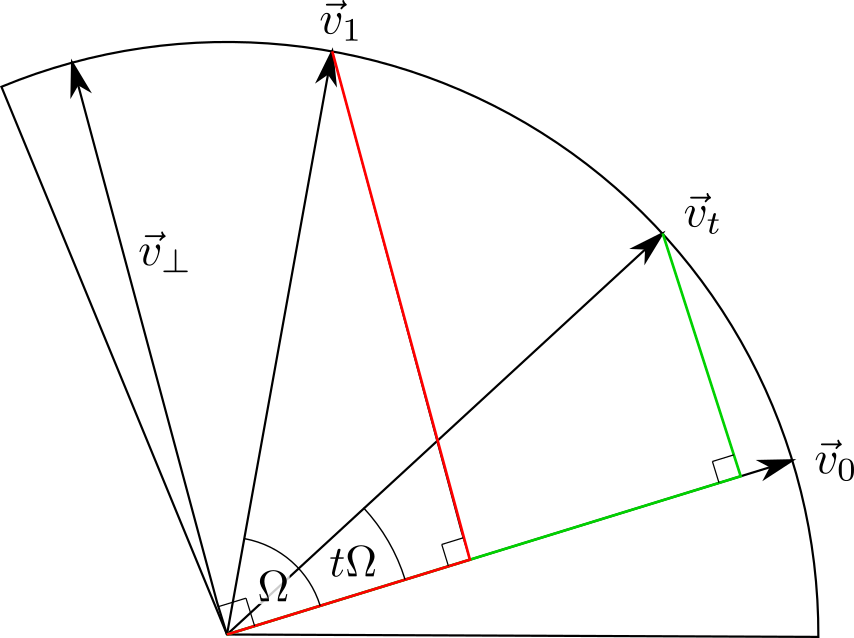
From the diagram:
\[\begin{align} \vec{v}_1 &= \color{red}{\cos\Omega \vec{v}_0 + \sin\Omega \vec{v}_{\perp}} \\ \therefore \vec{v}_{\perp} &= \frac{1}{\sin\Omega} (\vec{v}_1 - \cos\Omega \vec{v}_0) \end{align}\]Substitute in the expression for $\vec{v}_t$:
\[\begin{align} \vec{v}_t &= \color{green}{\cos (t \Omega )\vec{v}_0 + \sin (t\Omega ) \vec{v}_{\perp}} \\ &= \cos (t \Omega )\vec{v}_0 + \frac{ \sin (t\Omega )}{\sin\Omega}(\vec{v}_1 - \cos\Omega \vec{v}_0) \\ &= \frac{ 1 }{\sin\Omega}((\cos (t \Omega )\sin\Omega -\sin (t\Omega )\cos\Omega )\vec{v}_0 + \sin (t\Omega ) \vec{v}_1 )\\ &= \frac{ 1 }{\sin\Omega}(\sin(\Omega -t\Omega)\vec{v}_0 + \sin (t\Omega ) \vec{v}_1 ) \end{align}\]To convert this formula to 3D, replace the vectors with quaternions. That is all:
\[\begin{align} \text{slerp}(q_0, q_1, t) &= \frac{ 1 }{\sin\Omega}(\sin(\Omega -t\Omega)q_0 + \sin (t\Omega ) q_1 ) \\ \cos\Omega &= q_0 \cdot q_1 = s_0s_1 + x_0x_1 + y_0y_1 + z_0z_1 \end{align}\]This formula is used in the graph at the top and is the most common formula in quaternion animations. Please see the reference for a formal proof.
My informal explanation is: this formula can be seen as the linear addition of four parts: real, $i$, $j$ and $k$. The real part will cancel out in $qvq^{*}$. The other parts will undergo the same transformation as the 2D complex part $iy$ in $\vec{v} \equiv z = x + iy$, resulting in three circular interpolations that combined form the interpolation across a sphere.
Formula 2
Using Euler’s formula:
\[z_1 = z_0 e^{i \Omega}\]Substitute in the expression for $z_t$:
\[\begin{align} z_t &= z_0 e^{it \Omega} \\ &= z_0 (e^{i\Omega})^t \\ &= z_0 \left( \frac{z_1}{z_0} \right)^t \end{align}\]In quaternion form:
\[\text{slerp}(q_0, q_1, t) = q_0 (q_0^{-1} q_1)^t = q_0 (q_0^{*} q_1)^t\]More detail: proving the slerp formulas are equal ⇩
Conclusion
Thank you for following me along this journey into the fascinating mathematics of quaternions. I hope you’ve enjoyed it and are fully comfortable with using them in animations now.
Please explore the references in part 1 for more information.