Introduction to quaternions and rotations in 3D.
Update 11 December 2021: This post was featured on HackerNews and briefly held the top spot. Please see this link for the full discussion. Minor modifications have been done based on the comments.
This is part of a series. The other articles are:
This is a mathematical series and the following prerequisites are recommended: trigonometry, algebra, complex numbers, Euclidean geometry and linear algebra (matrices).
Table of Contents
- Animating in 3D
- Mathematical representations of rotations in 3D
- Outline
- Extra: Other forms of axis-angle rotations
- References
Quaternions
Animating in 3D
A common problem in computer animations is rotating an object in fully 3D space. Think objects, spaceships and heroes tumbling and turning in complex sequences. This is usually accomplished with an arcane mathematical object called a quaternion.1 For example, here is a spaceship rotating in Unity, a popular game engine that is often used to make mobile games:
The code to implement this uses Unity’s inbuilt Quaternion, making it very succinct:
var t = Time.time * speed;
transform.rotation = Quaternion.Slerp(init.rotation, final.rotation, t);
In Unity’s UI the init and final rotations are specified by three angles, which are then transformed into quaternions in the backend. This means that printing a rotation will result in four numbers, not three.
What are these four numbers? Unity’s own documentation is very elusive on what quaternions are. It is worth quoting it:
Quaternions are used to represent rotations.
They are compact, don't suffer from gimbal lock and can easily be interpolated. Unity internally uses Quaternions to represent all rotations.
They are based on complex numbers and are not easy to understand intuitively. You almost never access or modify individual Quaternion components ...
This is a common caveat next to the descriptions of properties:
Don't modify this directly unless you know quaternions inside out.
I did not encounter quaternions in all my years of engineering, although a lecturer once alluded to them during a class in my masters. They are frowned upon in favour of more intuitive and versatile vectors and matrices. Those can also be used to calculate 3D rotations and that is an approach that I did use in engineering, especially in my masters.
So why then are computer game developers and animators left to battle with this obscure mathematics that engineers won’t touch? Unity gives good reasons: compactness (4 numbers), numerical stability (“don’t suffer from Gimbal lock”) and interpolation (easy to find rotations between other rotations).2 These are significant differentiating factors in computer games and animations, which may need to compute many thousands of rotations every frame.
This series of posts seeks to illuminate quaternions so that you are one of those people who knows them “inside out”. Later posts will build the logical foundations for quaternions and describe the mathematics in detail. For the meantime, the rest of this post will be an interactive review of rotation methods in 3D.
Mathematical representations of rotations in 3D
There are two main methods to describe 3D rotations:
- Three angles and an order.
- An axis with three co-ordinates and an angle.
In both cases four quantities are used to describe the rotation, but usually one degree of freedom is fixed. For three angles, the order is fixed. For the axis-angle representation, the axis is set to have a unit length, so it can only exist on the unit sphere and hence two numbers are sufficient to describe it (latitude and longitude). In either case, there are three remaining degrees of freedom.
1. Three angles and an order
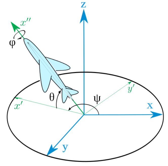
An intuitive way to describe a rotation is with three separate angles. These are known as the Euler angles after the great mathematician Leonhard Euler. There are many different conventions for Euler angles depending on the axes and orders chosen. For the interactive graph I have used the Tait-Bryan angle representation, which is often used in engineering. Here is an illustration:
The three angles are:
- $\psi$: yaw, about the $z$ axis.
- $\theta$: pitch, about the $y’$ axis3
- $\phi$: roll, about the $x’’$ axis.
The order used is yaw-pitch-roll, also called $\psi$-$\theta$-$\phi$ or $z$-$y’$-$x’’$ or ZYX. As an example of how the order affects the final rotation, here are two rotations done with a yaw of 30° and a roll of 90°. The left uses the yaw-roll order and the right a roll-yaw order.
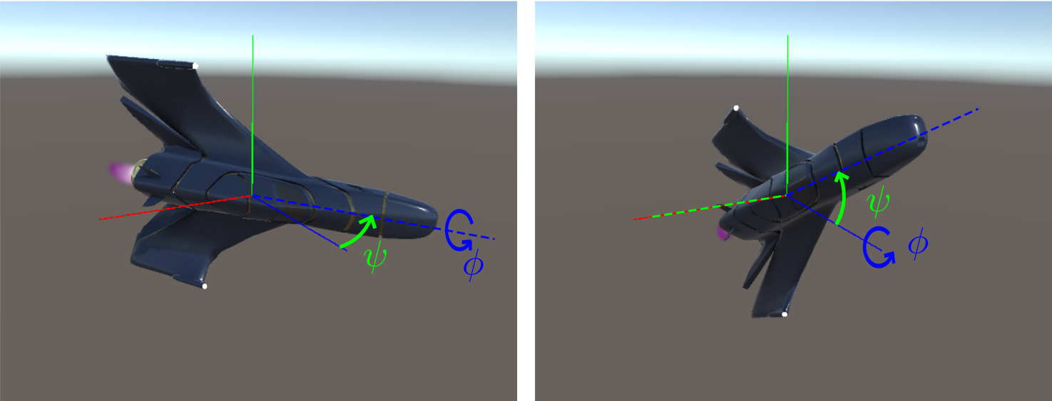
On the left, the cruiser first rotates 30° to the left and then rolls on its side. On the right, the cruiser rolls on it side first, so that a pilot sitting inside would perceive his left as up, and hence the yaw rotation results in a 30° movement upwards. This is why the order needs to be specified.
Given the order, each angle can be used to construct a 3×3 rotation matrix $R_{\alpha}$ which represents a 2D rotation about an axis. See part 2 for more detail. Then the rotated vector $v_r$ is obtained from $v$ by multiplying each matrix in order:
\[v_r = R_{\phi}R_{\theta}R_{\psi}v\]Matrix definitions
\[ R_{\psi} = \begin{bmatrix} \cos(\psi) & -\sin(\psi) & 0 \\ \sin(\psi) & \phantom{+}\cos(\psi) & 0 \\ 0 & 0 & 1 \end{bmatrix} \] \[ R_{\theta} = \begin{bmatrix} \phantom{+}\cos(\theta) & 0 & \sin(\theta) \\ 0 & 1 & 0 \\ -\sin(\theta) & 0 & \cos(\theta) \end{bmatrix} \] \[ R_{\phi} = \begin{bmatrix} 1 & 0 & 0 \\ 0 & \cos(\phi) & -\sin(\phi) \\ 0 & \sin(\phi) & \phantom{+}\cos(\phi) \end{bmatrix} \]
I would like to emphasise that the above graph is dynamically generated by using this equation to update the 3D co-ordinates for the Plotly charting library. The result is a natural looking rotation.4 The JavaScript code can be found here or with your browser’s inspection tools.
If you do follow the order, the base will rotate about one circle of the gimbal at a time. But what if you don’t follow it? For example, you move $\theta$ and $\phi$ before $\psi$? Go back and try this if you haven’t already. The answer is, the whole gimbal rotates to the orientation where it would have been if the rotation order of $z$-$y’$-$x’’$ was respected. This path cannot be represented with the angles $\psi$, $\theta$ or $\phi$. (It can be with other Euler angles but that only shifts the problem.) This already illustrates one of the biggest problems with Euler angles: it enforces unnatural constraints.
To see how this can create complexity, consider the interpolation problem in the initial GIF of this post. Given the angles for the first and final rotation, how would you find the rotation at the middle point?
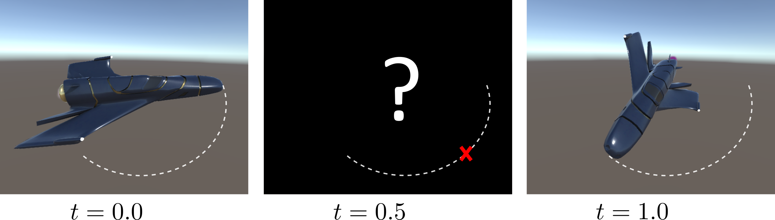
First make a circle that connects the nose of the cruiser from its starting position to its final position. Then for each point on the arc of the circle, find some $\psi$, $\theta$ and $\phi$ applied in that order that will result in a rotation to that point. This requires adjusting three angles simultaneously. One can imagine an algorithm where you adjust $\psi$, then $\theta$ then $\phi$ and if the point doesn’t fall on the circle where it is supposed to go, start from the beginning at $\psi$ again. A better algorithm is provided below, but it is still constrained by the same underlying process. We’ll see shortly that the quaternion algorithm is much, much simpler.
More detail: interpolation with Euler angles ⇩
- Using the inner product: $\cos(\alpha) = \vec{p}_0 \cdot \vec{p}_1 = x_1 x_2 + y_1 y_2 + z_1 z_2 $
-
The equation of the circle is $\vec{p}_t = r\cos(\alpha t)\hat{x} + r\sin(\alpha t)\hat{y}$
- Define $r = \lvert \vec{p}_0 \rvert = \lvert \vec{p}_1 \rvert $
- Define $\hat{x} = \frac{1}{r}\vec{p}_0 $
- Calculate $\hat{y}$ from $\vec{p}_1 = r\cos(\alpha)\hat{x} + r\sin(\alpha)\hat{y}$
- With (2) there is enough information to create the animation, but what if we want the angles? This requires solving 3 highly non-linear trigonometric equations from $p_t=R_{\phi}R_{\theta}R_{\psi}p_0$. An alternative is to calculate an axis-angle rotation matrix with $\hat{n} = \hat{x} \times \hat{y}$ and $\theta = \alpha t$. Then compare terms with the Euler rotation matrix.
Another problem comes from gimbal lock. This is not an issue when the rotations are enforced, which is the situation in animations. But going the other way, where rotations need to be calculated from accelerations and velocities - as is often the case in physics problems - this is a major problem. In particular, when the pitch is 90°, yaw and roll switch, and this provides enough ambiguity in the equations to inject significant numeric instability. (The same happens at a 90° angle for yaw and roll but only the middle angle causes a problem.) For this reason, Euler angles should never be used in physics simulations - I speak from experience.
More detail: proving gimbal lock ⇩
Concluding this section, we have discovered that Euler angles are intuitive and work well for static systems. However they are not suited for dynamic systems, whether that be through interpolation or numerical integration. Thankfully the next method does work well in the latter case.
2. An axis and an angle
q = +1.000 + 0.000i + 0.000j + 0.000k
Note that every point on the circle can be reached twice: through the clockwise rotation or through the anti-clockwise rotation. This is known as the double cover property.
There are multiple ways to calculate the axis-angle representation. This graph uses a quaternion. See the source code here or with your browser’s inspection tools.
What is a quaternion? Here is a mathematical definition:
Definition: Quaternion
/kwəˈtəːnɪən/
A quaternion is a number of the form $$s + xi+yj + zk \; ; \; s, x, y, z \in \mathbb{R}$$ where the basis elements $i$, $j$ and $k$ obey the following rules of multiplication: $$i^2 = j^2 = k^2 = ijk = -1 \;,\; ij=k \;,\; ji=-k$$
It may be unusual that $ij=k$ but $ji=-k$, but this should not be surprising after the Euler angles section. 3D rotations depend on order and hence any mathematics that represents them must depend on order. Part 3 will provide further physical justifications for this abstract definition.
The quaternion is calculated from the normal vector and $\theta$ as follows:
\[\begin{aligned} \hat{n} &= \cos(\beta)\cos(\alpha)i + \cos(\beta)\sin(\alpha)j + \sin(\beta)k \\ q &= \cos(\tfrac{\theta}{2}) + \sin(\tfrac{\theta}{2})\hat{n} \end{aligned}\]The rotation is then done with this formula (proved in part 3):
\[\begin{aligned} v_r &= qvq^{*}\\ &= (\cos (\tfrac{\theta}{2}) + \sin (\tfrac{\theta}{2})\hat{n})v(\cos (\tfrac{\theta}{2})- \sin (\tfrac{\theta}{2}) \hat{n}) \end{aligned}\]Euler angles are 3D which we can visualise, while quaternions are 4D which means we cannot. Why then should we prefer quaternions? Their main advantage comes with interpolations. Here again is the problem of finding the middle rotation between the starting and final rotations in the GIF:
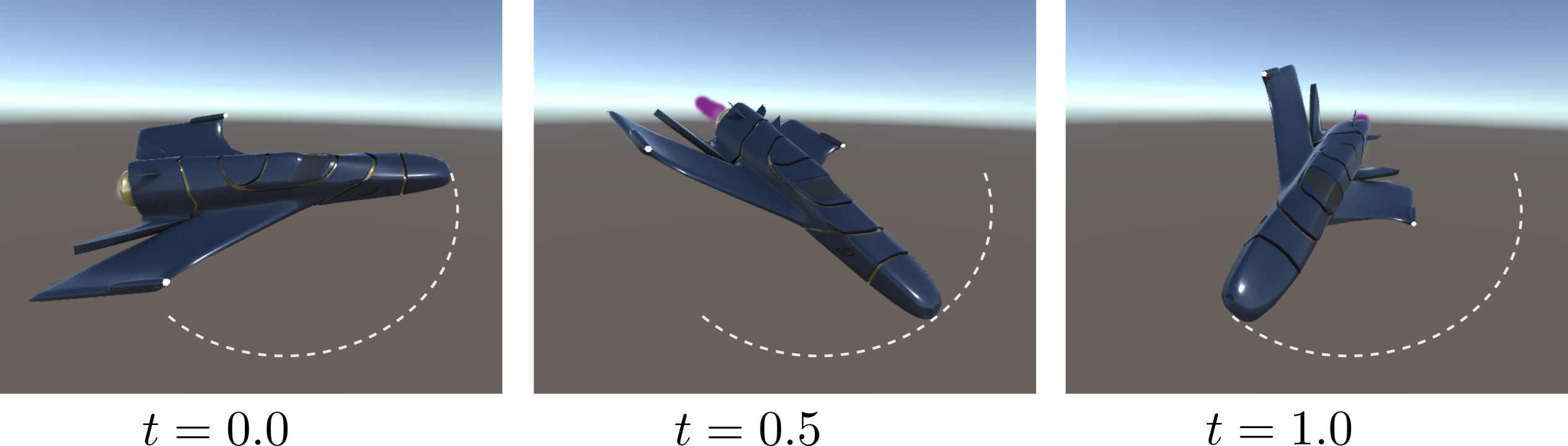
Again we draw the arc of a circle which the nose of the cruiser will travel along. The axis-angle representation is a natural fit to this problem, because this arc can itself be represented with a normal vector and an angle. Even so, the quaternion solution to the problem is unexpectedly simple. For this special case of $t=0.5$, calculate the quaternion:
\[q_{0.5} = \frac{q_{0.0} + q_{1.0}}{2}\]and apply the rotation formula. Done.
In general the expression for $q_t$ is more complex. But I hope this example gives a sense of the power of quaternions.
Outline
Using quaternions for 3D rotations is a very sensible choice for animation software. They are essentially an array of four numbers with the normal rules for addition and subtraction and some special rules for multiplication. Encode that, and you get rotation functions and stateless, fast, interpolations almost for free.
I hope this post has illuminated some of their properties and advantages. If you wish to learn more, the rest of the series will expand more on the mathematics of quaternions.
- Part 2 describes rotations in 2D. It describes complex numbers, which can be thought of as a simpler type of quaternion.
- Part 3 describes the fundamentals of quaternions and their mathematics. A few proofs of their properties are given.
- Part 4 focuses on interpolation. An interactive graph with a stick aeroplane in place of the Unity space cruiser is presented.
To get the most out of this series, you should be comfortable with trigonometry, algebra, complex numbers, Euclidean geometry and linear algebra (matrices). This maths was covered in my first year of engineering.
This series is the kind I would have liked to see. When I first learnt about quaternions I found that I had to consult many sources to understand them properly. Nearly every source began with a story of an Irish mathematician, a bridge, and an epiphany that caused him to carve the fundamental formula of quaternions into the stone. It’s a nice story but it is a confusing one to begin with. Why did he have this epiphany? What “magic” did he grasp that day and can we also? In part 3 I do tell this story, but at a point where sufficient mathematics has been discussed so we can somewhat approximate the mathematician’s thoughts that day. Instead I chose to lead with a different story; one about why quaternions are still relevant 178 years later. I hope this was appreciated.
This series is written from the perspective of an engineer. I try to introduce ideas and justify them in as intuitive a way as possible. Mathematical proofs are only done for identities where that is difficult. I also do not explore how quaternions fit into the general context of mathematical fields and algebras, or more general versions of quaternion algebra.
Extra: Other forms of axis-angle rotations
Identical rotations could also be accomplished with other formulas, namely the Rodrigues’ formulas and with Pauli matrices. I will give the formulas without going into detail; this is only to compare forms.
The Rodrigues’ formulas are as follows:
\[\begin{aligned} \vec{v}_r &= \cos \theta \vec{v}+ \sin \theta (\hat{n} \times \vec{v}) + (1-\cos \theta)(\vec{v} \cdot \hat{n}) \hat{n} \\ \vec{v}_r &= [I_3 + \sin\theta N + (1-\cos \theta) N^2]\vec{v} \;, \; N\vec{v} = \hat{n} \times \vec{v} \end{aligned}\]Note that $\vec{v} = (x, y, z)^T \equiv 0 + xi + yj + zk = v$.
The Pauli matrices formula is a sort of intermediate form between quaternions and the Rodrigues formulas. It uses 2×2 matrices and complex numbers:
\[\begin{aligned} \vec{v} \cdot \vec{\sigma} &= \begin{bmatrix} z & x + iy \\ x - iy & -z \end{bmatrix} \\ U &= \cos (\tfrac{\theta}{2}) I_2 - \sin (\tfrac{\theta}{2})(i\hat{n} \cdot \vec{\sigma}) \\ \vec{v}_r \cdot \vec{\sigma} &= U(\vec{v} \cdot \vec{\sigma} ) U^\dagger \end{aligned}\]Here again is the quaternion formula:
\[\begin{aligned} v_r &= qvq^{*}\\ &= (\cos (\tfrac{\theta}{2}) + \sin (\tfrac{\theta}{2})\hat{n})v(\cos (\tfrac{\theta}{2})- \sin (\tfrac{\theta}{2}) \hat{n}) \end{aligned}\]These are four different formulas which are based on four different branches of mathematics (Euclidean geometry, linear algebra and complex numbers, quaternions) with multiple different types of multiplications (scalar multiplication, quaternion multiplication, dot products, vector cross products and matrix multiplication), yet these formulas all represent the same physical rotation and will result in identical vectors $\vec{v}_r$.
For a comparison of all formulas in Julia, please see this repository: Rotations.
Quaternions are best for interpolations and hence animations. But any of these methods will work for physics simulations. Personally, I have successfully used the Rodrigues matrix formula on simulations of complex 3D robots.
More detail: axis-angle formulas from angular velocities ⇩
References
There are many sources I used to learn about quaternions. Each provides more detail in some area, whether it be animations, mathematical formulas, or visualisations.
- Quaternions, Interpolation and Animation by Erik B. Dam, Martin Koch and Martin Lillholm (1998): a comprehensive guide of quaternion mathematics and how to use them in animations. The main source material for this series.
- Quaternion Algebras by John Voight (2021): a complete textbook on Quaternion Algebras. It shows that quaternions as used in animations are a choice within a larger group of similar algebras. It presents many elegant proofs for the properties of quaternions. It quickly goes beyond normal quaternions and most certainly this author’s knowledge.
- Representing Attitude: Euler Angles, Unit Quaternions, and Rotation Vectors by James Diebel (2006): a concise guide to Euler angles and quaternions, with formulas for many different kinds and conversion formulas between each type.
- Visualizing quaternion by Grant Sanderson and Ben Eater: a stunning interactive website with tutorials on visualising 4 dimensional quaternions in 3 dimensions through stereographic projections.
- Dirac’s belt trick, Topology, and Spin ½ particles by Noah Miller: an interesting video on the applications of 3D rotations in quantum mechanics. I encountered the Pauli matrices rotation formula for the first time in this video.
- Wikipedia: comprehensive articles on quaternions and related subjects.
- Wired article on quaternions: a brief history of quaternions, their old rivalry with vectors and their impact.
-
It is quaternion for the Latin word for 4, quattuor. Before knowing any better, I assumed it was quartonion for the anglicized word “quarter”. ↩
-
Interpolation between rotations imposes kinematics without regards to the physics. In engineering it is often the other way round: physics defines the kinematics. In other words, an applied force changes the orientation of an object. This often follows a highly non-linear profile. For example, a strong jerk might cause the object to twist suddenly from one rotation to the next. Interpolation meanwhile sets the rotations, like an invisible hand guiding the object, often with linear schemes resulting in smooth animations. ↩
-
Note: $z’$ points downwards so that positive $\theta$ is clockwise. ↩
-
Let’s get meta for a moment. Plotly itself gives you the ability to rotate the entire plot. How does it do that? It uses the Tait-Bryan angles with the same order used here. The relevant functions from the source code are
rotateX,rotateYandrotateZ. ↩