Transformers for natural language processing from first principles. This a long post which details a full implementation of transformers and the mathematics behind them. The use case is predicting Amazon review stars based on the review text. The language of choice is Julia utilising the Flux machine learning framework.
Update 19 August 2023: code refactoring and update to Flux 0.13.11 explicit syntax.
Update 23 March 2024: code refactoring.
Update 2 February 2025: update to Flux 0.16.
See also: Generative transformer from first principles in Julia.
All code available at github.com/LiorSinai/TransformersLite.jl.
Table of Contents
Introduction
In December 2017 Google AI released their transformer architecture in the paper Attention is all you need. (It is a highly recommended read.) They had achieved state of the art results on an English to German translation task using a mostly linear model that could be easily scaled up and parallelized. Since then it has come to dominate the machine learning space. Many of the state of the art natural language processing (NLP) models today are transformer models. Most of them have an incredibly similar architecture to the original and differ only on training regimes, datasets and sizes.
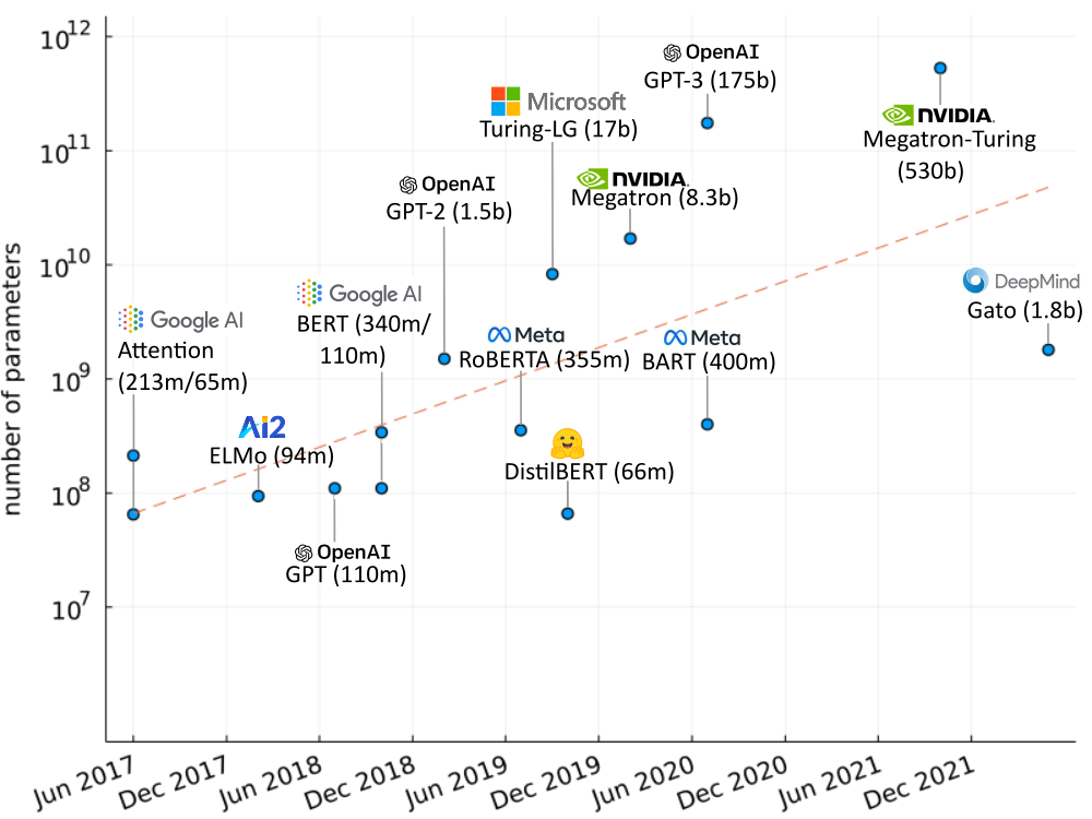
Transformers lend themselves to large models. The original transformer model was no light weight: it had 65 million parameters and could be scaled up to 213 million for marginal improvements. But this is tiny in comparison to OpenAI’s GPT-3 with 175 billion parameters. It is licensed over an API and is responsible for generating text that has made its way around the internet and popular science articles. These large models are even shaping hardware. The CEO of chip manufacturer Nvidia, Jensen Huang, focused a segment of his 2022 keynote speech on transformers and their impact on his industry. Nvidia have also released their own large transformer model with 530 billon parameters and have conducted tests with a 1 trillion parameter model.
Despite being originally developed for NLP, they have come for computer vision too. This 2020 paper showed that they can compete with top convolutional neural networks (CNNs). More recently, DeepMind released an impressive model Gato that can perform multiple tasks such as “play Atari, caption images, chat, stack blocks with a real robot arm and much more”. It has 1.8 billion parameters.
Goals
All this development in transformers has been over the past 5 years. Recurrent neural networks (RNNs) used to be the favourite for NLP in academia and industry yet transformers have almost replaced them in this short time frame. However it has not been long enough for pedagogy to adapt. As of today, machine learning courses still teach RNNs for NLP. This has created a gap and many blogs have sprung up to full it. This blog post aims to be one of those.
I have two goals here:
- Build a small working transformer in Julia code and train it on one use case.
- Detail the mathematics of the transformer for both forward equations and backpropagation.
Julia has a small but growing user base. It is an elegant and fast language and I highly recommend it. But even if you don’t know it well, I hope you will find this post accessible and that it will help improve your Julia. Mathematics on the other hand is a universal language and this should be accessible to anyone with university level maths.
The use case is a dataset of Amazon reviews from HuggingFace. Only the English subset of the dataset was used with 200,000 training samples and 5,000 test samples. The models were trained on two tasks:
- Predict the star rating given the review text.
- Predict a positive or negative sentiment with 1-2 stars labelled negative, 4-5 stars labelled positive and 3 stars removed.
This problem can be solved with simpler models e.g. a term frequency inverse document frequency (TFIDF) model with 10,000 parameters. (You can see my Julia TFIDF model here.) Using a transformer for this task can therefore be seen as excessive. However because the task is simple it means we can limit the transformer model to around 250,000 parameters and we have a good baseline of the accuracy we can achieve.
For intuition and history behind transformers I recommend Peter Bloem’s excellent post Transformers from scratch. For code in a more popular framework I recommend Alexander Rush’s The annotated transformer written in PyTorch. Many transformer posts focus on another universal language, pictures. Amongst the most notable are Jay Alammar’s the illustrated transformer and a video by Ari Seff. I’ll use pictures too but it won’t be the primary medium.
This is not meant to be a full scale Julia solution. For that, please see the Transformers.jl package. It has better optimizations, APIs for HuggingFace and more. My own repository with the code in this blog post can be accessed at github.com/LiorSinai/TransformersLite.jl.
Lastly, transformers are built on top of research and ideas of the last decade of machine learning research. A background in neural networks is needed for this post. For my part, I’ll briefly explain the ideas behind techniques like word embeddings, skip connections, regularization and so on and provide some references. I also encourage you to research more on your own. It is also worth keeping in mind that machine learning is at its heart an empirical science, and a sufficient if maybe unsatisfactory answer for why most of these techniques are used is that they have given good results in the past.
Design
Design considerations
First it is important to look at the design considerations that the Google AI team prioritised.
In the current era of machine learning, the best outcomes have been achieved with bigger models and more data. To facilitate this, a new architecture should have fast execution times and allow for parallel execution.

Let’s consider a scale of linear to non-linear. In computer terms, fast means simple and simple means linear. On the other side is non-linear which is complex and slow. Machine learning as used today is mostly linear. Anyone who first studies it is surely a little overwhelmed with all the linear algebra and matrices. Some non-linearity is needed but research has found that one can get away with very little. For example, only non-linearity in activation functions. CNNs are more non-linear, mostly because of the strides of the kernels across images.

The other scale is parallel to sequential. The previous favourite for NLP, RNNs, were very sequential. This makes sense for language where words themselves are sequential and the location and order of words in a sentence is important. Yet transformers are mostly parallel. This enables computers to distribute computation across GPU cores and across clusters. To reconcile this with sequential language two techniques are used: position encoding and masking. In practice these “hacks” perform well enough to justify using a parallel model for sequential tasks.
Inputs and outputs
The input to a transformer is a sentence. For example “This camera works great!”. That is then processed into tokens.
Depending on the complexity desired, these tokens can represent words, punctuation, and subword pieces like suffixes. For examples:
[This, camera, work, ##s, great, !]. A simpler approach is to remove case and punctuation: [this, camera, works, great].
Each token is then associated with a series of weights called a word vector or a word embedding. For example, for our sentence:
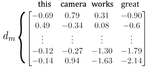
Each word has $d_m$ weights associated with it. For typical transformer models $d_m$ ranges from 64 to 2048. The main idea is that each weight represents some concept. For example if we were to assign them manually we could go according to this scheme:
- the first row is for how positive or negative the word is.
- the second row is for how common it is.
- the third row is for if it is a noun or not.
In practice these weights will be assigned during training and it can be hard to interpret them.
The output of the transformer is another set of weights usually of the same size:
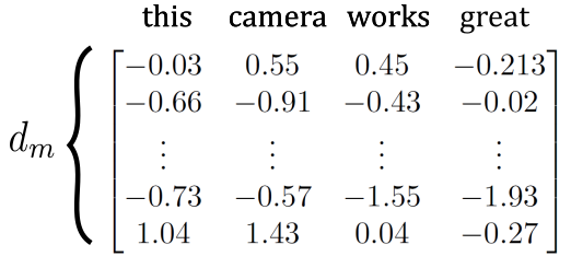
But now these weights have a different meaning. They are how each word relates to each other in the sentence and to the task at hand. Where as the previous weights were unique to each word, these are particular to a sentence. Change one word in the sentence and we might get a completely different matrix, depending on how important that word is. The name transformer comes from the fact that it transforms a set of word embeddings to another set of embeddings.
The transformer takes advantage of linear algebra to calculate all the weights for all words at the same time. Hence it is mostly a parallel computation. Without additional measures we could shuffle the words (columns) in the sentence and we would get shuffled versions of the same results. To parallelize further, we can stack the embedding matrices of sentences of $N$ words into $B$ batches of $d_m\times N \times B$ dimensional arrays.
Because the output looks like the input we can feed it back into another transformer. Transformer models tend to have stacks of 6 to 24 of these layers. With each layer it gets more difficult to interpret what the embedding weights actually mean. But stacking them has been shown to improve results.
The final output matrix is usually fed to a small neural network to output the final result. This could be a single number in the case of sentiment analysis or a probability of each word in a vocabulary for a translation task.
Architecture
This is the famous schematic from the paper Attention is all you need:
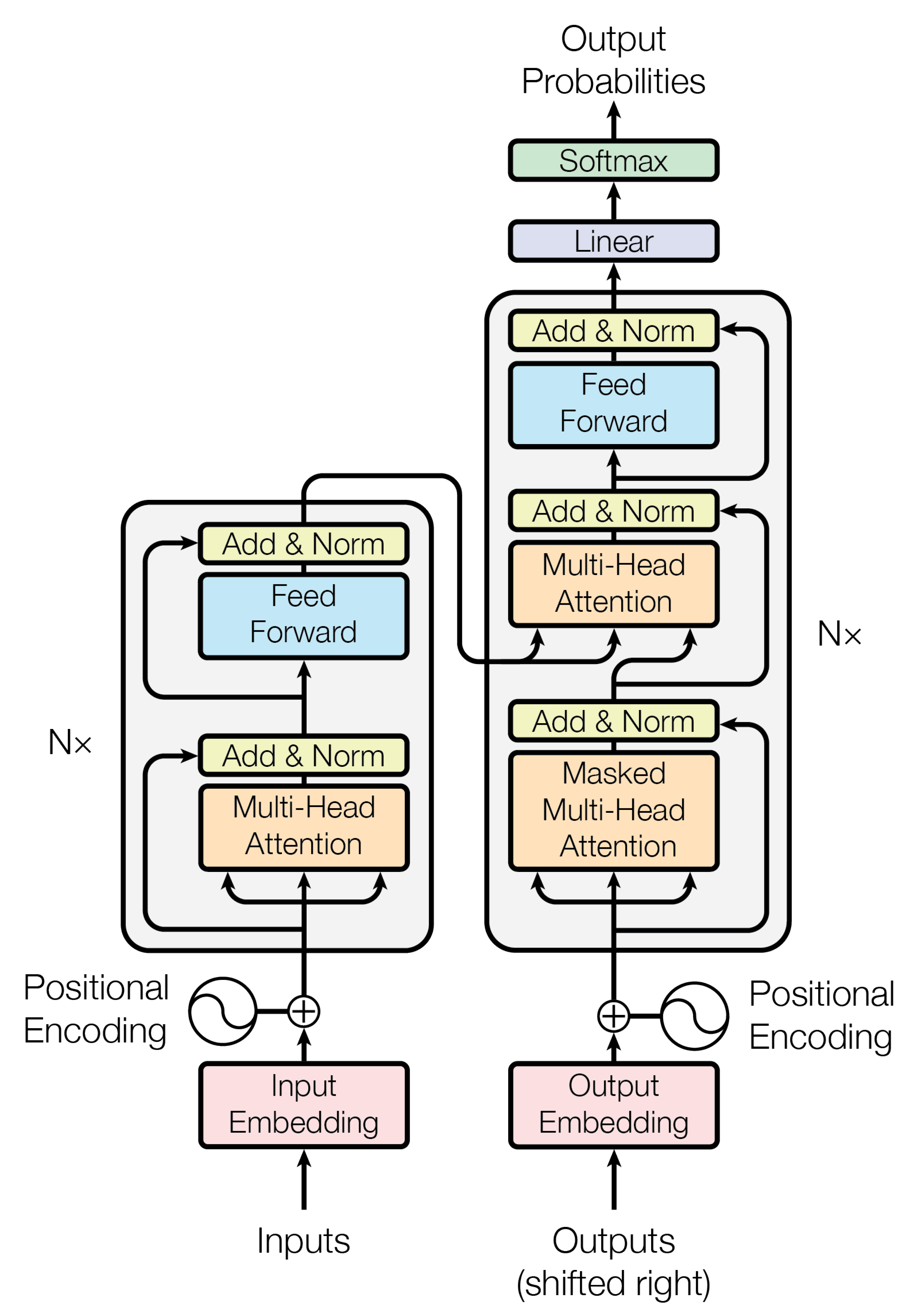
The left side is called an encoder and the right side a decoder. You don’t need both sides. BERT is an encoder-only model by Google. Gato is a decoder only transformer. In this post I’ll focus only on the encoder which is sufficient for the classification task.
Each block in the schematic is associated with two sets of equations: the forward equations and the backwards equations. I have compiled the encoder block equations into the table below. The task for the remainder of the blog post will be to translate this maths into code.
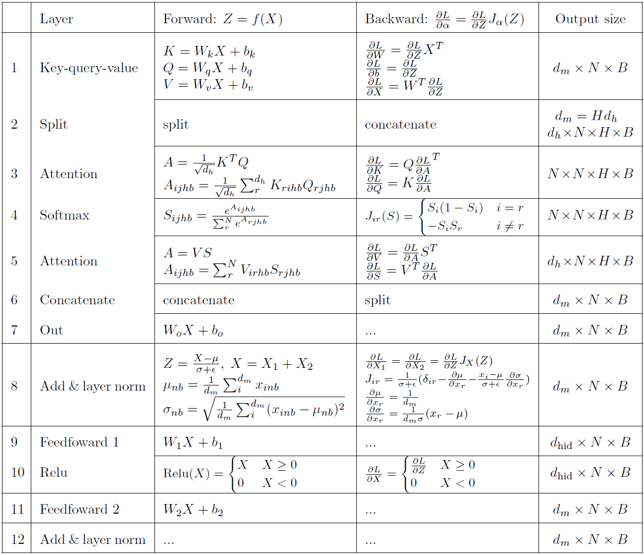
Please see this table only as a guideline. Some of the equations are incomplete so that they fit in this table. Equations will be presented properly in each subsection. $J_\alpha(Z)\equiv \frac{\partial Z}{\partial \alpha}$. There are 4 non-linear steps (softmax, 2×layer norm, RELU) and the other 8 are linear.
You’ll notice that the inputs are either 3D or 4D arrays. These are not standard in linear algebra so a section below is dedicated to getting comfortable with them. In particular, in any programming language multiplying two higher order arrays will not work. For example:
A = randn(3, 4, 2, 2)
3×4×2×2 Array{Float64, 4}:
[:, :, 1, 1] =
 0.539347   0.772838  0.793975  0.436097
 0.0890865  0.374346  0.462195  0.691458
 0.364314   0.701065  0.712357  0.801697
[:, :, 2, 1] =
 0.587629  0.128034  0.908577  0.221286
 0.526123  0.788315  0.692201  0.99606
 0.510707  0.338502  0.832025  0.33279
[:, :, 1, 2] =
 0.163337  0.991491   0.309396  0.155
 0.785946  0.0787799  0.160141  0.212985
 0.323122  0.806226   0.228209  0.205507
[:, :, 2, 2] =
 0.0339063  0.402629  0.239698   0.471303
 0.787614   0.8888    0.0176223  0.957667
 0.352839   0.153378  0.829512   0.256615
 -1.79658    1.45127   -1.11244
B = randn(4, 3, 2, 2);
A * B # MethodError: no method matching *(::Array{Float64, 4}, ::Array{Float64, 4})
Multiplication simply isn’t defined for them. So we’ll have to write our own function to handle the multiplication here and also for the backpropagation. We’ll do this as a simple extension to 2D matrix multiplication.1
Attention
The most important steps in the above table are the steps 3 to 5. Combing them into one and working with only 2D matrices, we get the definition for the scaled dot product attention:
\[A = V\text{softmax}\left(\frac{1}{\sqrt{d_h}}K^T Q\right)\]Where $\text{softmax}$ is the function:
\[\text{softmax}(z, i) = \frac{e^{z_i}}{\sum^N_r e^{z_r}}\]Attention is essentially a dot product of every column vector of the embedding matrix with some scaling. To see this more clearly, substitute the equations for $K$ and $Q$ into $K^TQ$ and ignore the bias:
\[K^T Q = (W_KX)^T(W_QX) = X^T W_K^T W_Q X\]I hope the $X^TX$ is recognisable as a dot product/inner product. The Google authors call it a different name, attention, and it is apparently all you need. It is very closely related to an older machine learning technique called cosine similarity.
Every word is multiplied with the embeddings of every other word, resulting in a small $N \times N$ matrix. The hope is that the output looks something like:
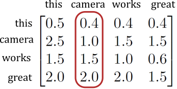
Reading down the columns we have an approximate weighting of how much every word thinks every other word is important. Or in the paper’s terms, how much each word is paying attention to every other word. Here “camera” thinks “great” is the most important word in the sentence. Because of the weights this matrix is not symmetrical. So “great” actually places less importance on “camera” than “camera” places on it.
This matrix is at the heart of transformer. All the other layers work towards it or aim to use weights output by it.
Julia implementation
Project setup
We’ll be making use of the Flux framework along with the NNlib and ChainRulesCore packages.
An example output will be:
TransformerClassifier(
  Embedding(32 => 7455),                # 238_560 parameters
  PositionEncoding(32),
  Dropout(0.1),
  [
    TransformerBlock(
      MultiHeadAttention(
        nhead=4,
        denseQ = Dense(32 => 32; bias=false),  # 1_024 parameters
        denseK = Dense(32 => 32; bias=false),  # 1_024 parameters
        denseV = Dense(32 => 32; bias=false),  # 1_024 parameters
        denseO = Dense(32 => 32),       # 1_056 parameters
      ),
      LayerNorm(32),                    # 64 parameters
      Dense(32 => 128, relu),           # 4_224 parameters
      Dense(128 => 32),                 # 4_128 parameters
      LayerNorm(32),                    # 64 parameters
      Dropout(0.1),
    ),
  ],
  Dense(32 => 1),                       # 33 parameters
  FlattenLayer(),
  Dense(50 => 5),                       # 255 parameters
)         # Total: 18 trainable arrays, 251_456 parameters,
          # plus 1 non-trainable, 32_000 parameters, summarysize 1.082 MiB.
The Dropout, LayerNorm and Dense layers are already part of the Flux package.
We’ll be making Embed, PositionEncoding, MultiheadAttention, TransformerEncoderBlock and FlattenLayer.
We’ll also make a small index tokenizer to map tokens to word vectors.
The focus will be on the forward equations because Flux handles the backwards equation through automatic differentiation (AD). Other than reducing our job in half, AD also means our forward and backwards equations will always be in sync. There will be collapsible blocks with backpropagation information.
To start, make a package in the Julia REPL:
cd("path\\to\\project\\directory")
] # enter package mode
generate TransformersLite # make a directory structure
activate TransformersLite # activate package environment
add Flux NNlib ChainRulesCore
activate
dev "path\\to\\project\\directory\\TransformersLite"
The goal of using the package manager is that we can now use the super helpful Revise package, which will dynamically update most changes during development without errors:
julia> using Revise
julia> using TransformersLite
To follow this tutorial, it is recommended to load the dependencies directly:
using Flux
using NNlib
using ChainRulesCore
You can see my final code at github.com/LiorSinai/TransformersLite.jl. This is based loosely on the registered Transformers.jl package.
Tokenizers
The input is a sentence that we need to break up into tokens. This preprocessing step is a huge topic itself and I am not going to go into too much detail.
We will be making a fixed set of embeddings in the next section. That means we need to work from a fixed vocabulary list in this section. Any word that is not in this vocabulary will be marked as “unknown” and will have minimal impact on the output.
Firstly it is recommended to simplify the text to reduce the diversity of tokens. The following function converts everything to lowercase, normalises letters (e.g. è to e) and removes punctuation (including “don’t” to “dont”):
using Unicode

function simplify(s::AbstractString)
    s = lowercase(s)
    s = Unicode.normalize(s, :NFD)
    s = replace(s, r"['`’\u200d\p{M}]" => "")
    s = replace(s, r"\n" => " ")
end
Then we can use the following function to create a vocabulary list:
using DataStructures

function select_vocabulary(corpus::AbstractVector{<:AbstractString};
    min_document_frequency::Int=10, pattern::Regex=r"\w\w+\b", transform=simplify)
    document_frequencies = DefaultDict{String, Int}(0)
    for document in corpus
        words = Set{String}()
        for m in eachmatch(pattern, transform(document))
            word = m.match
            if !(word in words)
                push!(words, word)
                document_frequencies[word] += 1
            end
        end
    end
    filter!(x->x[2] ≥ min_document_frequency, document_frequencies)
    vocab = collect(document_frequencies)
    sort!(vocab, by=x->x[2], rev=true)
    [v[1] for v in vocab]
end
I’ve already created such a list of 6653 words for the Amazon reviews task:
amazon_reviews_train_en.txt.
These are words which are present in at least 30 different reviews.
Note that the vocabulary is sorted from highest to lowest of the document frequencies in the original data.
So if we limit the vocabulary e.g. vocab[1:1000] we can still be confident that it will have statistical significance.
The load_vocab function is used to load the words:
function load_vocab(filepath::AbstractString)
    vocab = String[]
    open(filepath, "r") do file
        for line in eachline(file)
            push!(vocab, line)
        end
    end
    vocab
end
vocab = load_vocab("amazon_reviews_train_en.txt")
The next step is to break the text into words. This is best done with a regular expression:
pattern = r"\w\w+\b"
words = map(m->string(m.match), eachmatch(pattern, document))
Putting it together:
text = "This coffee from Kenya is really good."
tokens = map(m->string(m.match), eachmatch(pattern, simplify(text)))
tokens # [this,coffee,from,kenya,is,really,good]
An optional step after this is subword tokenization.
I have made simple tokenizers for this at github.com/LiorSinai/TokenizersLite.jl.
You can also use the registered BytePairEncoding.jl package.
If you do not want subword tokenization use tokenizer=identity and the tokens will be the words themselves.
That is sufficient for the Amazon Reviews problem that we will investigate later.
Once we have tokens we need to map them to word embeddings.
For this we’ll make a simple IndexTokenizer which will do the following:
indexer = IndexTokenizer(vocab, "[UNK]")
tokens = ["this","coffee","from","kenya","is","really","good"]
indices = indexer(tokens) # [8,534,50,1,6,56,30]
Now for the IndexTokenizer. Start with the constructor:
struct IndexTokenizer{T}
    vocabulary::Vector{T}
    lookup::Dict{T, Int}
    unksym::T
    unkidx::Int
    function IndexTokenizer(vocab::Vector{T}, unksym::T) where T
        if !(unksym ∈ vocab)
            pushfirst!(vocab, unksym)
            unkidx = 1
        else
            unkidx = findfirst(isequal(unksym), vocab)
        end
        lookup = Dict(x => idx for (idx, x) in enumerate(vocab))
        new{T}(vocab, lookup, unksym, unkidx)
    end
end

Base.length(tokenizer::IndexTokenizer) = length(tokenizer.vocabulary)

function Base.show(io::IO, tokenizer::IndexTokenizer)
    T = eltype(tokenizer.vocabulary)
    print(io, "IndexTokenizer{$(T)}(length(vocabulary)=$(length(tokenizer)), unksym=$(tokenizer.unksym))")
end
This IndexTokenizer takes in the vocabulary list and an unknown symbol.
The constructor function checks if the unknown symbol is in the list else it adds it to the front.
It also creates a reverse lookup from words to indices.
This doubles space requirements but greatly speeds up processing.
For the encoding process we replace a token with an index if it is in the vocabulary list otherwise we use the unknown symbol index (by default 1):
function encode(tokenizer::IndexTokenizer{T}, x::T) where T
    if haskey(tokenizer.lookup, x)
        return tokenizer.lookup[x]
    end
    tokenizer.unkidx
end
This assumes we are giving a single token of type T.
We also want to do multiple dispatch on sentences which are Vector{T} and on batches of sentences which are Vector{Vector{T}}.
When working with batches we’ll need all sentence to be the same length.
Here the unknown token is used for padding:
function encode(tokenizer::IndexTokenizer{T}, seq::AbstractVector{T}) where T
    map(x->encode(tokenizer, x), seq)
end

function encode(tokenizer::IndexTokenizer{T}, batch::AbstractVector{Vector{T}}) where T
    lengths = map(length, batch)
    indices = fill(tokenizer.unkidx, maximum(lengths), length(batch))
    for (i, seq) ∈ enumerate(batch)
        for (j, x) ∈ enumerate(seq)
            @inbounds indices[j, i] = encode(tokenizer, x)
        end
    end
    indices
end
Lastly we can add a method to do multiple dispatch on the type IndexTokenizer itself,
which turns this struct into a function:
(tokenizer::IndexTokenizer)(x) = encode(tokenizer, x)Word embeddings
Word embeddings were already introduced in the Inputs and Outputs section. Here we’ll make a simple layer to store and retrieve them.
It it worth highlighting that the word embedding is unique to each model and will be trained from random values for each model. This is not how humans work. Part of what makes language so useful is that we have generic connotations and meanings for words and then derive more specific meaning from them in a given context. For example, the word “good” always has the same “embedding” in any context. But here we learn a different embedding for different models and even different training runs.
There are several justifications for this:
- Word embeddings are task specific: for example in the Amazon review context “return” is a highly negative word associated with returning a defective product to the store. In other tasks it may be far more neutral.
- The tokenizer strategy from the previous section might change, or we might want to experiment with different tokenizers.
- We can tune the model dimension $d_m$ as a hyperparameter to make bigger or smaller models.
This is somewhat unfortunate as it forms a massive part of our training. For the model we will use later it will be 95% of the trainable parameters.
The embedding layer is a struct that holds a matrix:
struct Embed{W <: AbstractArray}
    weight::W
end

Flux.@layer Embed # tell Flux that this struct is trainable

Embed(output_dim::Int, vocab_size::Int) = Embed(randn(Float32, output_dim, vocab_size))

Base.size(e::Embed) = size(e.weight)

Base.show(io::IO, e::Embed) = print(io, "Embed($(size(e.weight)))")
The Float32 type is used to reduce the size of the model and for performance benefits. We don’t need the extra accuracy provided by Float64.
We have a second show function for multimedia (MIME) types when we went prettier printing e.g. in the REPL and Jupyter notebooks.
The Flux.@functor Embed line is essential for Flux to be able to perform backpropagation.
For the forward pass we will use NNlib.gather:
using NNlib: gather
function (e::Embed)(x::AbstractArray{Int})
    gather(e.weight, x)
end
This is equivalent to e.embedding[:, x]. However gather is slightly more versatile and comes with the benefit of already having an rrule defined for it (source):
∇gather_src(Δ, src_size, idx) = scatter!(+, fill!(similar(Δ, eltype(Δ), src_size), 0), Δ, idx)The rrule is a reverse (backwards) rule that encodes the derivative for backpropagation.2
It is what makes the magic of automatic differentiation work.
The function gather does not have a formal derivative, but scatter is the opposite of it and is what we need to apply when we calculate the loss:
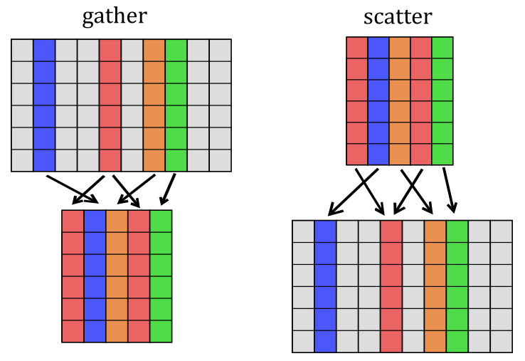
At the end of backpropagation we need to distribute the error matrix amongst the original word embeddings.
This is what scatter does. Note that we use the red column twice, so we have two error columns directed towards it.
The rrule applies + as the reducing function; that is, the two errors are added together and then to the word embedding.
Scatter is very inefficient. If we do a small experiment and call scatter we will see it results in a large matrix of mostly zeros:3
NNlib.scatter(+, rand(8, 4), [1, 5, 11, 1]; dstsize=(8, 15))
8×15 Matrix{Float64}:
 1.62703   0.0  0.0  0.0  0.495725  0.0  0.0  0.0  0.0  0.0  0.237452     0.0  0.0  0.0  0.0
 0.979735  0.0  0.0  0.0  0.984499  0.0  0.0  0.0  0.0  0.0  0.145738     0.0  0.0  0.0  0.0
 0.892948  0.0  0.0  0.0  0.76959   0.0  0.0  0.0  0.0  0.0  0.714658     0.0  0.0  0.0  0.0
 1.45113   0.0  0.0  0.0  0.883492  0.0  0.0  0.0  0.0  0.0  0.52775      0.0  0.0  0.0  0.0
 0.702824  0.0  0.0  0.0  0.965256  0.0  0.0  0.0  0.0  0.0  0.0966964    0.0  0.0  0.0  0.0
 1.16978   0.0  0.0  0.0  0.568429  0.0  0.0  0.0  0.0  0.0  0.000161501  0.0  0.0  0.0  0.0
 1.80566   0.0  0.0  0.0  0.271676  0.0  0.0  0.0  0.0  0.0  0.430018     0.0  0.0  0.0  0.0
 1.16445   0.0  0.0  0.0  0.911601  0.0  0.0  0.0  0.0  0.0  0.786343     0.0  0.0  0.0  0.0
Position encodings
As mentioned before, the matrix operations on the embedding matrix are parallel operations. They do not take order into account. One of the proposed methods proposed in the Attention is all you need paper to counteract this is to add constant value “position encodings” to the matrix. The hope is that the model will learn these constant values and hence the relative and absolute positions. For example a simple choice for each column $j$ is $\frac{j}{n_{max}}$:
\[\begin{bmatrix} \frac{1}{n_{max}} & \frac{2}{n_{max}} & \cdots & \frac{n_{max}-1}{n_{max}} & 1 \\ \vdots & \vdots & \ddots & \vdots & 1 \\ \frac{1}{n_{max}} & \frac{2}{n_{max}} & \cdots & \frac{n_{max}-1}{n_{max}} & 1 \end{bmatrix}\]A problem with this encoding is that it is dependent on the parameter $n_{max}$ which fixes the sequence length. Instead the authors propose a more convoluted solution but one that can be easily scaled to any sequence length:
\[\begin{align} PE(2i + 1, j) &= \sin(j/(10^4)^{2i/d}) \\ PE(2i + 2, j) &= \cos(j/(10^4)^{2i/d}) \end{align}\]Plotted here on the left is a heatmap of the resultant matrix and on the right are the sine waves used for the odd numbered rows:
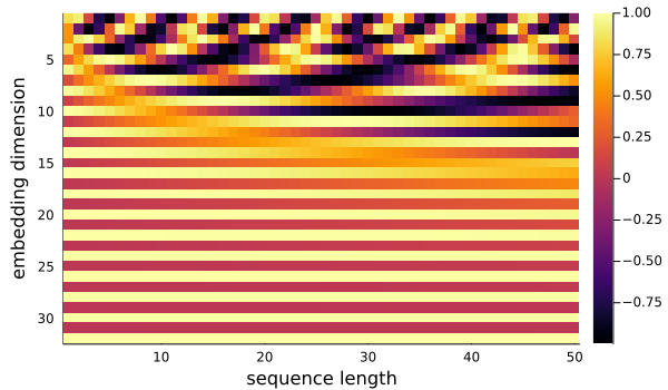
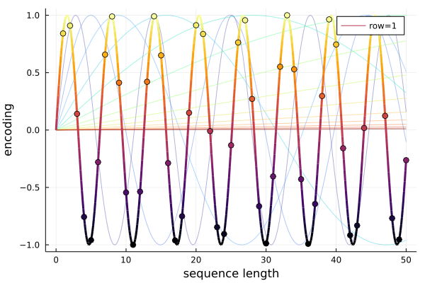
Each column has a unique pattern so the encoding does accomplish its task. To understand how, lets focus on the first row with $i=0$. This sine wave has a wavelength of $2\pi \approx 6.28$ and we sample it every $1$ time step so it repeats every 6 blocks. This leads to the 6 alternating colours in the top row: 3 light, then 3 dark, then repeat. So this sine wave can distinguish between sequences of length 6 or less. Now let’s move on to $i=1$. This sine wave has a period of $2\pi(10^4)^{2/32} \approx 11.17$ so it repeats approximately every 11 blocks in the 3rd row. We can now distinguish between sequences of up to length 11 and we can use the first row for greater precision. As we add sine waves, we can distinguish between sequences of longer wave lengths. In general the wavelengths are $2\pi(10^4)^{2i/d}$.
The remaining question is why use both sine and cosine waves? The answer in the paper is: “We chose this function because we hypothesized it would allow the model to easily learn to attend by relative positions, since for any fixed offset $k$, $PE_{j+k}$ can be represented as a linear function of $PE_{j}$.” Here they are referring to the identities:
\[\sin(\omega k + \omega j) = \sin(\omega k)\cos(\omega j) + \cos(\omega k)\sin(\omega j) \\ \cos(\omega k + \omega j) = \cos(\omega k)\cos(\omega j) + \sin(\omega k)\sin(\omega j) \\\]which are linear for constant $\omega$ and $k$. For more detail please see here.4
Now let’s code the PositionEncoding layer.
Since these values are constant it is easiest to preallocate a matrix:
struct PositionEncoding{W <: AbstractArray}
    weight::W
end

#= make this layer discoverable by Flux but specify no weights are trainable =#
Flux.@layer PositionEncoding trainable=()

function PositionEncoding(dim_embedding::Int, max_length::Int=1000)
    W = make_position_encoding(dim_embedding, max_length)
    PositionEncoding(W)
end

function make_position_encoding(dim_embedding::Int, seq_length::Int, n::Int=10000)
    encoding = Matrix{Float32}(undef, dim_embedding, seq_length)
    for pos in 1:seq_length
        for row in 0:2:(dim_embedding - 1)
            denom = 1/(n^(row/dim_embedding))
            encoding[row + 1, pos] = sin(pos * denom)
            encoding[row + 2, pos] = cos(pos * denom)
        end
    end
    encoding
end

function Base.show(io::IO, pe::PositionEncoding)
    print(io, "PositionEncoding($(size(pe.weight, 1)))")
end
The forward pass then selects the required columns from the pre-allocated array:
(pe::PositionEncoding)(x::AbstractArray) = (pe::PositionEncoding)(size(x, 2))
function (pe::PositionEncoding)(seq_length::Int)
    max_length = size(pe.weight, 2)
    if seq_length > max_length
        error("sequence length of $seq_length exceeds maximum position encoding length of $max_length")
    end
    pe.weight[:, Base.OneTo(seq_length)]
end
Here an error is raised if the size of the pre-allocated matrix is exceeded. We could instead calculate the extra columns required or resize the encoding matrix. For now this only adds extra complexity.
Also note this layer only returns the encoding, so we need to add it separately:
X = rand(32, 100, 16)
pe = PositionEncoding(32)
Z = X .+ pe(X) # broadcast the 2D encoding matrix to 3D
If desired we can move the addition into the forward pass e.g. for use in Flux.chain.
Multiplication with higher order arrays
Starting in 2D, matrix multiplication for $A\times B$ is defined as the sum of rows in $A$ multiplied with the columns in $B$:
\[C_{ij} = \sum_r A_{ir} B_{rj}\]This can be written as a set of three loops (ignoring checks):5
function mul2d(A<:AbstractMatrix, B<:AbstractMatrix)
	n = size(A, 2) # == size(B, 1)
	C = zeros(size(A, 1), size(B, 2))
	for i in 1:size(A, 1)
		for j in 1:size(B, 2)
			for r in 1:n
				C[i, j] += A[i, r] * B[r, j]
			end
		end
	end
	C
end
Of course many programming languages already have this function built in and have highly optimised it. We can do a quick time test:
A = randn(100, 100);
B = randn(100, 100);
@time mul2d(A, B); # 0.002391s
@time A * B;       # 0.000265s
The naive implementation is 9× slower. One of the reasons is the indexing is very inefficient. The code will start at the top and count down to the cell needed for each multiplication when we could take advantage of the fact that the next cell is next door:
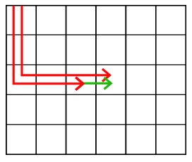
Later in machine learning came the idea of batch multiplication. This is doing multiplications for a set of independent matrices simultaneously by grouping them into one large 3D array:
\[C_{ijk} = \sum_r A_{irk} B_{rjk}\]We could write this as a set of four loops.
Or since we know the inbuilt * is faster we can substitute that for the three inner loops:
function mul3d(A::AbstractArray{T, 3}, B::AbstractArray{T, 3}) where T
    C = Array{Float64}(undef, size(A, 1), size(B, 2), size(A, 3))
    for k in 1:size(A, 3)
        C[:, :, k] = A[:, :, k] * B[:, :, k]
    end
    C
end
But this doesn’t take advantage of the fact that we are standardising the size of the matrices (all sequences are of the same length).
It is equivalent to using type Vector{Matrix{T}} rather than Array{T, 3}.
NNlib has written a more optimised version called batched_mul.
Doing a time test:
Using NNlib
A = randn(100, 100, 32);
B = randn(100, 100, 32);
@time mul3d(A, B);       # 0.010918s
@time batched_mul(A, B); # 0.006588s
The NNlib function is about 1.5× faster.
For transformers we work with 4D arrays but they are sets of sets of independent matrices (repetition intended). So multiplication is a set of five loops or two outer loops and matrix multiplication:
\[C_{ijkl} = \sum_r A_{irkl} B_{rjkl}\]function mul4d(A::AbstractArray{T, 4}, B::AbstractArray{T, 4}) where T
C = Array{Float64, 4}(undef, size(A, 1), size(B, 2), size(A, 3), size(A, 4))
for l in 1:size(A, 4)
for k in 1:size(A, 3)
C[:, :, k, l] = A[:, :, k, l] * B[:, :, k, l]
end
end
C
endmul4d it will not work:
y, pull = Flux.pullback(mul4d, A, B);
errors = randn(size(y)...);
grads = pull(errors)rrule for it.
Backpropagation is well known for a linear layer: $$ \frac{\partial L}{\partial W} = \frac{\partial L}{\partial Z} X^T \\ \frac{\partial L}{\partial X} = W^T \frac{\partial L}{\partial Z} $$ Here are two good derivations using different techniques: 1 (chain rule) and 2 (Jacobian). If take away the special meanings of weights $W$ and features $X$ we have a general rule for $A\times B$ where $A=W$ and $B=X$. We can extend this to 3D and 4D without going through a formal proof by noting that the matrices are independent of each other. Hence the equations are: $$ \frac{\partial L}{\partial A}_{ijkl} = \sum_r \frac{\partial L}{\partial Z}_{irkl} B_{jrkl} \\ \frac{\partial L}{\partial B}_{ijkl} = \sum_r A_{rikl} \frac{\partial L}{\partial Z}_{rjkl} $$ where the transpose is done by swapping the indices. Thankfully there is an inbuilt function to do the transposition in higher order arrays:
PermutedDimsArray. So the rrule is relatively short:
import ChainRulesCore.rrule
using ChainRulesCore: @thunk, NoTangent
function rrule(::typeof(mul4d), A::AbstractArray{T, 4}, B::AbstractArray{T, 4}) where T
    C = mul4d(A, B)
    function mul4d_pullBack(C̄)
            Ā = @thunk mul4d(C̄, PermutedDimsArray(B, (2, 1, 3, 4)))
            B̄ = @thunk mul4d(PermutedDimsArray(A, (2, 1, 3, 4)), C̄)
        return NoTangent(), Ā, B̄
    end
    return C, mul4d_pullBack
endusing Flux.)
Making an optimised version of this is beyond the scope of this post.
But what we can do is extend batched_mul by reshaping 4D $m\times n \times p \times q$ arrays into 3D $m\times n \times pq$ arrays:
import NNlib.batched_mul
function batched_mul(A::AbstractArray{T, 4}, B::AbstractArray{T, 4}) where {T}
    if (size(A, 2) != size(B, 1)) || (size(A, 3) != size(B, 3)) || (size(A, 4) != size(B, 4))
        message = "A has dimensions $(size(A)) but B has dimensions $(size(B))"
        throw(DimensionMismatch(message))
    end
    new_A = reshape(A, size(A, 1), size(A, 2), :)
    new_B = reshape(B, size(B, 1), size(B, 2), :)
    C = batched_mul(new_A, new_B)
    new_C = reshape(C, (size(C, 1), size(C, 2), size(A, 3), size(A, 4)))
    new_C
end
Doing a time test
A = randn(50, 50, 12, 32)
B = randn(50, 50, 12, 32)
@time mul4d(A, B);       # 0.016885
@time batched_mul(A, B); # 0.005216s
The batched_mul version is about 3× faster.
We don’t need to write a rrule for it because rules already exists for reshape and batched_mul.
Multi-head attention
We are finally at the heart of the transformer: multi-head attention.
At the end of this step we will have a MultiheadAttention layer:
MultiheadAttention(
  nhead=4,
  denseQ = Dense(32 => 32; bias=false),  # 1_024 parameters
  denseK = Dense(32 => 32; bias=false),  # 1_024 parameters
  denseV = Dense(32 => 32; bias=false),  # 1_024 parameters
  denseO = Dense(32 => 32),             # 1_056 parameters
)                  # Total: 5 arrays, 4_128 parameters, 16.422 KiB.
The multi-head attention layer splits up the embedding matrix into multiple heads. Each head will act on an embedding dimension of $d_h$ instead of the full $d_m$ as if the embedding was only $d_h$ in size. If we have $H$ heads then $d_m=Hd_h$.
First define a struct to hold all the dense layers and a parameter for $H$ called nhead:
struct MultiheadAttention{Q<:Dense, K<:Dense, V<:Dense, O<:Dense}
    nhead::Int
    denseQ::Q
    denseK::K
    denseV::V
    denseO::O
end

#= # tell Flux which parameters are trainable =#
Flux.@layer :ignore MultiheadAttention trainable=(denseQ, denseK, denseV, denseO)
We would like $d_m$ to be divisible by $H$ but the maths will work if it is not. So if the user supplies $d_h$ accept it as valid:
function MultiheadAttention(nhead::Int, dim_model::Int, dim_head::Int, dim_out::Int)
    MultiheadAttention(
        nhead,
        Dense(dim_model, dim_head*nhead; bias=false),
        Dense(dim_model, dim_head*nhead; bias=false),
        Dense(dim_model, dim_head*nhead; bias=false),
        Dense(dim_head*nhead, dim_out),
    )
end

function MultiheadAttention(
    nhead::Int, dim_model::Int, dim_out::Int
    )
    if dim_model % nhead != 0
        error("embedding dimension=$dim_model is not divisible by number of heads=$nhead")
    end
    MultiheadAttention(nhead, dim_model, div(dim_model, nhead), dim_out)
end
Define printing functions:
function Base.show(io::IO, mha::MultiheadAttention)
    dh = div(size(mha.denseQ.weight)[1], mha.nhead)
    dm = size(mha.denseQ.weight)[2]
    dout = size(mha.denseO.weight)[1]
    print(io, "MultiheadAttention(")
    print(io, "nhead=$(mha.nhead), ")
    print(io, "head_size=$(dh), ")
    print(io, "$(dm)=>$(dout)")
    print(io, ")")
end

function Flux._big_show(io::IO, mha::MultiheadAttention, indent::Int=0)
    inner_indent = indent + 2
    print(io, " "^indent, "MultiheadAttention(\n")
    println(io, " "^inner_indent, "nhead=$(mha.nhead),")
    Flux._layer_show(io, mha.denseQ, inner_indent, "denseQ")
    Flux._layer_show(io, mha.denseK, inner_indent, "denseK")
    Flux._layer_show(io, mha.denseV, inner_indent, "denseV")
    Flux._layer_show(io, mha.denseO, inner_indent, "denseO")
    print(io, " "^indent, ")")
    if indent == 0
        Flux._big_finale(io, mha)
    else
        println(io, ",")
    end
end
Now let’s start with the forward pass. We first calculate a query, key and value from the input matrix. These terms are kind of archaic. They refer to a database model where the user makes a query (text in a search box), this is mapped to keys (video titles) and a value is returned (video). Or for a more direct programming metaphor: a hashmap where the query is hashed to a key to retrieve a value. The matrix multiplications here represent a softer version of this where we are returning a weighting of the values. The same matrix is used as the query, key and value, which can be interpreted as a self-reflective lookup, analogous to asking a query what it thinks is most important about itself.
But the names aren’t so important.
The query, key and value are each calculated using the dense matrices we stored in the struct based on the input matrices.6
Then we calculate the attention for all the heads at once with multi_head_scaled_dot_attention.
The final result is passed to the dense output layer:
function (mha::MultiheadAttention)(query::A3, key::A3, value::A3) where {
    T, A3 <: AbstractArray{T, 3}}
    # batch multiplication version. Input is dm × N × B
    Q = mha.denseQ(query)
    K = mha.denseK(key)
    V = mha.denseV(value)
    A = multi_head_scaled_dot_attention(mha.nhead, Q, K, V)
    mha.denseO(A)
end
The multi_head_scaled_dot_attention begins as follows:
function multi_head_scaled_dot_attention(nhead::Int, Q::A3, K::A3, V::A3) where {
    T, A3 <: AbstractArray{T, 3}}
    qs = size(Q)
    ks = size(K)
    vs = size(V)
    dm = size(Q, 1)
    dh = div(dm, nhead)
The $Q$, $K$ and $V$ matrices need to be split from $d_m \times N \times B$ to $d_h \times N \times H \times B$. This is done in two steps:
- $(d_h \times H)\times N \times B$ (break $d_m$ into $d_h$ and $H$)
- $d_h \times N \times H \times B$ (swap the 2nd and 3rd dimensions)
    Q = permutedims(reshape(Q, dh, nhead, qs[2], qs[3]), [1, 3, 2, 4])
    K = permutedims(reshape(K, dh, nhead, ks[2], ks[3]), [1, 3, 2, 4])
    V = permutedims(reshape(V, dh, nhead, vs[2], vs[3]), [1, 3, 2, 4])
Then we calculate the scaled dot attention for each head, combine results (undo the splitting) and return it:
    A = scaled_dot_attention(Q, K, V)
    A = permutedims(A, [1, 3, 2, 4])
    A = reshape(A, dm, size(A, 3), size(A, 4))
end
Using the batched_mul function from the previous section it is straightforward to calculate attention:7
function scaled_dot_attention(query::A1, key::A2, value::A3) where {
    T, A1 <: AbstractArray{T, 4}, A2 <: AbstractArray{T, 4}, A3 <: AbstractArray{T, 4}}
    # Batched version. Input is (dh, N, nhead, B)
    dh = size(query, 1)
    keyT = permutedims(key, (2, 1, 3, 4))
    score = one(T)/convert(T, sqrt(dh)) .* batched_mul(keyT, query)
    score = softmax(score; dims=1) #size(score) == (N, N, nhead, B)
    batched_mul(value, score) #size(attention) == (dh, N, nhead, B)
end
The softmax function (and its rrule) are provided by NNlib. For backpropagation information please see this link.
Notes on backpropagation in the attention layer ⇩
permutedims and batched_mul to get the same result.
The one last thing we need to do is make it work for a single embedding instead of a batch. For code reuse the best solution is to make a single embedding a batch of one:
function (mha::MultiheadAttention)(query::A1, key::A2, value::A3) where {
    T, A1 <: AbstractMatrix{T}, A2 <: AbstractMatrix{T}, A3 <: AbstractMatrix{T}}
    # single sample version. Input is dm × N
    query = reshape(query, size(query, 1), size(query, 2), 1)
    key   = reshape(key, size(key, 1), size(key, 2), 1)
    value = reshape(value, size(value, 1), size(value, 2), 1)
    A = mha(query, key, value)
    reshape(A, size(A, 1), size(A, 2))
end
Testing:
mha = MultiheadAttention(4, 32, 32)
q, k, v = rand32(32, 10, 4), rand32(32, 10, 4), rand32(32, 10, 4)
a = mha(q, k, v) # 32×10×4 Array{Float32, 3}
Encoder blocks
We still need to complete the rest of the equations in the table.
Thankfully the rest of the layers are provided by Flux. We wrap them in an TransformerEncoderBlock:
struct TransformerBlock{
    MHA<:MultiheadAttention,
    N1<:LayerNorm,
    D1<:Dense,
    D2<:Dense,
    N2<:LayerNorm,
    DO<:Dropout}
    multihead_attention::MHA
    norm_attention::N1
    dense1::D1
    dense2::D2
    norm_feedforward::N2
    dropout::DO
end
Flux.@layer TransformerBlock # make whole block trainable
This layer includes drop out regularization which wasn’t in the table but it is part of the original paper. During training this layer randomly sets some weights to zero. This interferes with training but makes it less likely to overfit. Have a look at these graphs from the training for the sentiment analysis task:
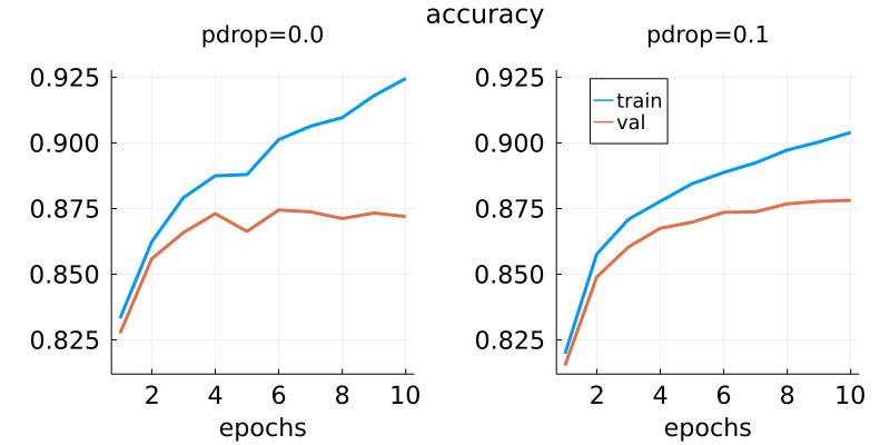
With 10% of dropout there is a much smaller gap between the validation and training accuracies.
Layer norm is a normalization over each layer. In the embedding matrix that is each word, so each column in each batch of matrices. There are other kinds of normalization like batch normalization, which is a normalization across batches. Interestingly layer norm was only popularised after batch normalization in this 2016 paper.
The function used for layer norm is:
\[a_{nb}\frac{X_{nb}-\mu_{nb}}{\sigma_{nb}+\epsilon} + b_{nb}\]for every column $n$ of every batch $b$. This has two parameters in $a_{nb}$ and $b_{nb}$.
They are not so important and you can turn them off with LayerNorm(d, affine=false).
$\epsilon$ is a small constant value for numerical stability.
For backpropagation information please see
my post.
Because the inputs and outputs are similar we only need four parameters to define the whole block:
TransformerBlock(nhead::Int, dm::Int, dhid::Int; pdrop::Float64=0.1) =
    TransformerBlock(
        MultiheadAttention(nhead, dm, dm),
        LayerNorm(dm),
        Dense(dm, dhid, relu),
        Dense(dhid, dm),
        LayerNorm(dm),
        Dropout(pdrop)
    )
Printing functions:
function Base.show(io::IO, block::TransformerBlock)
    print(io, "TransformerBlock(")
    print(io, block.multihead_attention)
    print(io, ", ", block.norm_attention)
    print(io, ", ", block.dense1)
    print(io, ", ", block.dense2)
    print(io, ", ", block.norm_feedforward)
    print(io, ")")
end
Lastly, the forward pass:
function (t::TransformerBlock)(x::A) where {A<:AbstractArray}
    h = t.multihead_attention(x, x, x) # (dm, N, B)
    h = t.dropout(h)
    h = x + h
    h = t.norm_attention(h)            # (dm, N, B)
    hff = t.dense1(h)                  # (dh, N, B)
    hff = t.dense2(hff)                # (dm, N, B)
    hff = t.dropout(hff)
    h = h + hff
    h = t.norm_feedforward(h)          # (dm, N, B)
    h
end
Skip connections are short-circuits. They look like they are undoing all the hard work of the previous layer. However these have proved very useful for neural networks with many layers because they carry a strong signal both on the forward pass and with the gradient on the backwards pass.
Testing:
block = TransformerBlock(4, 32, 64)
X = rand32(32, 10, 4)
Y = block(X) # 32×10×4 Array{Float32, 3}:
Classifier
At last, our model is almost ready for use.
There is just one last question, how to use the output embedding matrix?
We could do an aggregation on each word first to turn it into a matrix: $d_m \times N \times B \rightarrow N \times B$.
This aggregate could be a mean or a dense layer.
Or we could flatten the whole array into a $d_m N \times B$ matrix.
Either way this is followed by a Dense layer with $k \times B$ outputs for $k$ classes.
My preference is to aggregate on each word first with a dense layer. Here is a flatten layer which we will need to use to reduce the dimension: $1\times N \times B \rightarrow N \times B$.
struct FlattenLayer end

function (f::FlattenLayer)(x::AbstractArray{T, 3}) where T
  reshape(x, :, size(x, 3)) # same as Flux.flatten
end

function (f::FlattenLayer)(x::AbstractArray{T, 2}) where T
    reshape(x, :, 1) # returns a column vector
end
We can now make our model with Flux chain:
position_encoding = PositionEncoding(32)
add_position_encoding(x) = x .+ position_encoding(x)
model = Chain(
    Embed(32, 7455),
    add_position_encoding, # can also make anonymous
    Dropout(0.1),
    TransformerBlock(4, 32, 32 * 4; pdrop=0.1),
    Dense(32, 1),
    FlattenLayer(),
    Dense(50, 5)
    )
Test:
X = rand(1:7455, 50, 8)
Y = model(X) # 5×8 Matrix{Float32}
Alternatively see classifier.jl in the repository for a version of the same model wrapped in a struct with nicer printing and names. Making a model with this:
model = TransformersLite.TransformerClassifier(
    Embedding(7455 => 32),
    PositionEncoding(32),
    Dropout(0.1),
    TransformerBlock[
        TransformerBlock(4, 32, 32 * 4; pdrop=0.1)
    ],
    Dense(32, 1),
    FlattenLayer(),
    Dense(50, 5)
    )
Test:
X = rand(1:7455, 50, 8)
Y = model(X) # 5×8 Matrix{Float32}
Finally, we have a working transformer!
Use case: Amazon Reviews
Presented here is a subset of the results from scripts and notebooks at github.com/LiorSinai/TransformersLite.jl/tree/main/examples.
Data exploration
⚠️ WARNING: The dataset used here is no longer publicly available.
Download the data using HuggingFace’s Python API:
""" PYTHON CODE """
from datasets import load_dataset
dataset = load_dataset('amazon_reviews_multi', 'en', cache_dir='datasets')
You could download the raw data directly using curl:
curl https://amazon-reviews-ml.s3-us-west-2.amazonaws.com/json/train/dataset_en_train.json --output amazon_reviews_en_train
curl https://amazon-reviews-ml.s3-us-west-2.amazonaws.com/json/test/dataset_en_test.json --output amazon_reviews_en_test
However the HuggingFace API is nicer because it converts the array of JSONs to the more efficient and compact Arrow format.
The Amazon Reviews English dataset consists of 200,000 test samples and 5,000 training samples. The reviews are equally divided into 5 stars where 1 is a low score and 5 is best. There are eight features:
- review_id
- product_id
- reviewer_id
- stars
- review_body
- review_title
- language
- product_category
The models were only trained on “stars” and “review_body”.
A small sample of reviews (original spelling and punctuation):
| Star | Review |
|---|---|
| 5 | I like everything abut them they are perfect! |
| 4 | This is not a bad chair for the price. I had some problems with the wheels but they were promptly addressed by very helpful customer service. So overall I can give the 4 stars to this product. |
| 3 | As expected and average product |
| 2 | Overall quality is good on this product although they are smaller in size than anticipated. |
| 1 | Dissapointing, bad quality dont buy |
The reviews can go up to 4,000 characters, but most are much shorter than that:
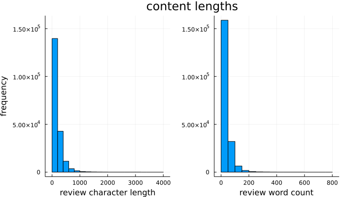
Of these reviews, 80% have less than 260 characters and/or less than 50 words. This justifies setting a maximum token count of 50.
Pipeline
Here is a pipeline for training a model, from tokenizing the input to saving the output data. This pipeline implements a rudimentary development workflow with:
- An output directory named after the date-time in “yyyymmdd-HHMM” format.
- Training history saved in JSON format.
- Hyperparameters that are used to control flow and are saved in JSON format.
The embedding dimension dim_embedding should be at least 8 for the Amazon Review task.
You might want to change nhead to 1 if you do use this value.
With a vocabulary of 6,000 words this results in a model with around 54,000 parameters.
It takes about 10 minutes to train on an Intel i7 CPU with 1.80 GHz processing power and 8GB of RAM.
Otherwise the default is an embedding dimension of 32 and 4 heads, which results in about 250,000 parameters.
This takes about 1 hour to train.
Results between the smaller and bigger models were almost identical, except the bigger model converged slightly faster.
Imports:
using Random
using DataFrames
using Arrow
using ProgressMeter
using Printf
using BSON, JSON
using Flux
using Flux: DataLoader
using Dates
using StatsBase: mean
using TransformersLite
Initialisation:
path = "datasets\\amazon_reviews_multi\\en\\1.0.0\\"
filename = "amazon_reviews_multi-train.arrow"
to_device = cpu # gpu or cpu

fingerprint = readdir(path)[1]
filepath = joinpath(path, fingerprint, filename)

df = DataFrame(Arrow.Table(filepath))
display(df)

hyperparameters = Dict(
    "seed" => 2718,
    "tokenizer" => "none",
    "nlabels" => 5,
    "pdrop" => 0.1,
    "dim_embedding" => 32
)
nlabels = hyperparameters["nlabels"]
Tokenizers (see the Tokenizers section):
path_vocab = joinpath("vocab", "amazon_reviews_train_en.txt")
tokenizer = identity
vocab = load_vocab(path_vocab)
indexer = IndexTokenizer(vocab, "[UNK]")
display(tokenizer)
display(indexer)
Tokens pipeline:
function preprocess(document::AbstractString, tokenizer;
    pattern::Regex = r"\w\w+\b", max_length::Union{Nothing, Int}=nothing, transform=simplify
    )
    words = map(m->string(m.match), eachmatch(pattern, transform(document)))
    tokens = tokenizer(words)
    if !isnothing(max_length)
        if length(tokens) > max_length
            tokens = tokens[1:max_length]
        end
    end
    tokens
end
documents = df[!, :review_body]
labels = df[!, :stars]
max_length = 50
@time tokens = map(d->preprocess(d, tokenizer, max_length=max_length), documents)
@time indices = indexer(tokens)
Train/validation data split.
function split_validation(
    rng::AbstractRNG, data::AbstractArray, labels::AbstractVecOrMat
    ; frac::Float64=0.1
    )
    nsamples = size(data)[end]
    idxs = randperm(rng, nsamples)
    ntrain = nsamples - floor(Int, frac * nsamples)
    inds_start = ntuple(Returns(:), ndims(data) - 1)
    ## train data
    idxs_train = idxs[1:ntrain]
    train_data = data[inds_start..., idxs_train]
    train_labels = ndims(labels) == 2 ? labels[:, idxs_train] : labels[idxs_train]
    ## validation data
    idxs_val = idxs[(ntrain + 1):end]
    val_data = data[inds_start..., idxs_val]
    val_labels = ndims(labels) == 2 ? labels[:, idxs_val] : labels[idxs_val]
    (train_data, train_labels), (val_data, val_labels)
end

y_train = copy(labels)
if nlabels == 1
    y_train[labels .≤ 2] .= 0
    y_train[labels .≥ 4] .= 1
    idxs = labels .!= 3
    y_train = reshape(y_train, 1, :)
else
    idxs = Base.OneTo(length(labels))
    y_train = Flux.onehotbatch(y_train, 1:nlabels)
end

X_train, y_train = indices[:, idxs], y_train[:, idxs];
rng = MersenneTwister(hyperparameters["seed"])
train_data, val_data = split_validation(rng, X_train, y_train)

println("train samples:      ", size(train_data[1]), " ", size(train_data[2]))
println("validation samples: ", size(val_data[1]), " ", size(val_data[2]))
Training
Model:
dim_embedding = hyperparameters["dim_embedding"]
pdrop = hyperparameters["pdrop"]
model = TransformersLite.TransformerClassifier(
    Embed(dim_embedding, length(indexer)),
    PositionEncoding(dim_embedding),
    Dropout(pdrop),
    TransformerEncoderBlock[
        TransformerEncoderBlock(4, dim_embedding, dim_embedding * 4; pdrop=pdrop)
    ],
    Dense(dim_embedding, 1),
    FlattenLayer(),
    Dense(max_length, nlabels)
    )
display(model)
model = to_device(model)

hyperparameters["model"] = "$(typeof(model).name.wrapper)"
hyperparameters["trainable parameters"] = sum(length, Flux.params(model));
Training helper functions.
The train! function is based off Flux.train! except it returns a history and uses the package ProgressMeter.
It is meant to be used with Flux.DataLoader for working with batched data.
function train!(loss, model, train_data, opt_state, val_data; num_epochs=10)
    history = Dict("mean_batch_loss" => Float64[])
    for epoch in 1:num_epochs
        print(stderr, "")
        progress = Progress(length(train_data); desc="epoch $epoch/$num_epochs")
        total_loss = 0.0
        for (i, Xy) in enumerate(train_data)
            batch_loss, grads = Flux.withgradient(model) do m
                loss(m(Xy[1]), Xy[2])
            end
            Flux.update!(opt_state, model, grads[1])
            total_loss += batch_loss
            ProgressMeter.next!(
                progress; showvalues =
                [(:mean_loss, total_loss / i), (:batch_loss, batch_loss)]
            )
        end
        mean_batch_loss = total_loss / length(train_data)
        push!(history["mean_batch_loss"], mean_batch_loss)
        update_history!(history, model, train_data, "train_", loss, accuracy)
        update_history!(history, model, val_data, "val_", loss, accuracy)
    end
    println("")
    history
end

function update_history!(history::Dict, model, data, prefix::String, funcs...)
    metrics = batched_metrics(model, data, funcs...)
    for func in keys(metrics)
        metric_name = prefix * String(func)
        if !(haskey(history, metric_name))
            history[metric_name] = [metrics[func]]
        else
            push!(history[metric_name], metrics[func])
        end
        @printf "%s=%.4f; " metric_name metrics[func]
    end
    println("")
end

function batched_metrics(model, data, funcs...)
    results = zeros(Float32, length(funcs))
    num_observations = 0
    @showprogress desc="batch metrics..." for (x, y) in data
        y_model = model(x)
        values = map(f->f(y_model, y), funcs)
        batch_size = count_observations(x)
        results .+= values .* batch_size
        num_observations += batch_size
    end
    results /= num_observations
    (; zip(Symbol.(funcs), results)...)
end

count_observations(data::D) where {D<:DataLoader} = count_observations(data.data)
count_observations(data::Tuple) = count_observations(data[1]) # assume data[1] are samples and data[2] are labels
count_observations(data::AbstractArray{<:Any,N}) where {N} = size(data, N)
count_observations(data) = length(data)
Training:
if nlabels == 1
    loss(x, y) = Flux.logitbinarycrossentropy(x, y)
    accuracy(ŷ, y) = mean((Flux.sigmoid.(ŷ) .> 0.5) .== y)
else
    loss(x, y) = Flux.logitcrossentropy(x, y)
    accuracy(ŷ, y) = mean(Flux.onecold(ŷ) .== Flux.onecold(y))
end

batch_size = 32
train_data_loader = DataLoader(train_data |> to_device; batchsize=batch_size, shuffle=true)
val_data_loader = DataLoader(val_data |> to_device; batchsize=batch_size, shuffle=false)

metrics = batched_metrics(model, val_data_loader, loss, accuracy)

@printf "val_acc=%.4f ; " metrics.accuracy * 100
@printf "val_loss=%.4f \n" metrics.loss

start_time = time_ns()
opt_state = Flux.setup(Adam(), model)
history = train!(
    loss,
    model,
    train_data_loader,
    opt_state,
    val_data_loader
    ; num_epochs=n_epochs
)
end_time = time_ns() - start_time
println("done training")
@printf "time taken: %.2fs\n" end_time/1e9
Save:
directory = "outputs\\" * Dates.format(now(), "yyyymmdd_HHMM")
mkdir(directory)

output_path = joinpath(directory, "model.bson")
history_path = joinpath(directory, "history.json")
hyperparameter_path = joinpath(directory, "hyperparameters.json")

model = model |> cpu
BSON.bson(
    output_path,
    Dict(
        :model=> model,
        :tokenizer=>tokenizer,
        :indexer=>indexer
    )
)

open(history_path,"w") do f
  JSON.print(f, history)
end

open(hyperparameter_path, "w") do f
    JSON.print(f, hyperparameters)
end
Evaluation
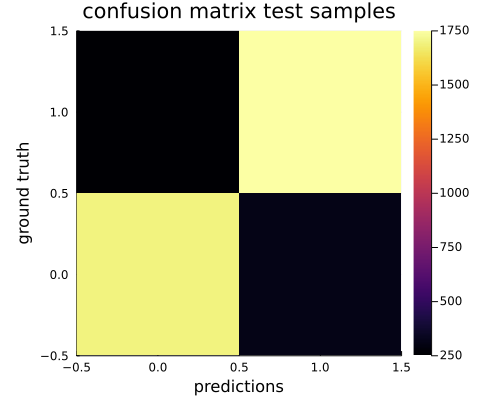
The accuracy achieved was 87.4% for the binary task and 49.9% for the 5 star classification task. This is up from a random baseline of 50% for the binary task and 20% for the 5 star classification task.
The confusion matrix shows that the binary model does indeed mostly predict the correct class:
A useful cross-section of the confusion matrix is the probabilities per each ground truth class:
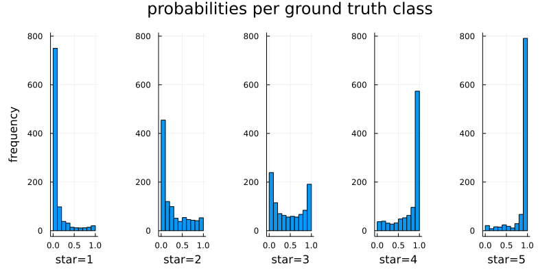
These distributions are mostly skewed in the correct way, with 1 star ratings being mostly negative and 5 star ratings mostly positive. The model was not trained on 3 star reviews so here the distribution is almost uniform (random) with a slight negative skew. However this may also be a reflection of the underlying data with humans not being consistent with their ratings for 3 stars.
Changing focus to the 5 star case:
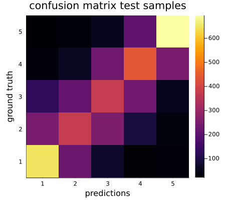
Looking at the confusion matrix we can see that the model struggles with the middle ratings of 2-4 but was mostly accurate with the extreme ratings of 1 and 5. Again this is hypothesized to be partially because of the underlying data.
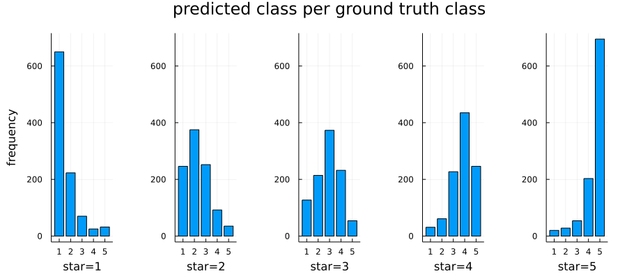
Seeing in another view as a bar chart, for each star the most likely prediction is the star itself. However the distributions do have a spread and leave significant overlap for confusion.
Although these results are not 100% perfect, it is a big achievement to have a model that can automatically attach sentiment to text.
Conclusion
Thank you for following this tutorial. I hope you now have a working transformer and have much better insight into how they work.
-
There is a set of multidimensional algebraic objects called tensors where multiplication is defined for higher orders. Confusingly, Google named their machine learning framework TensorFlow and calls higher order arrays tensors. So one should differentiate between machine learning tensors and geometric tensors. They are not the same. To give a simple explanation: one can think of geometric tensors as higher order arrays with severe constraints on their entries and operations because they represent geometric objects. These constraints make it harder - not easier - to code higher order arrays as geometric tensors.
For those who have studied tensors in physics: the multiplication output required is:
\[C_{ijk} = \sum_r A_{irk} B_{rjk}\]If we arbitrarily assign some co-ordinates as co-variant and some as contra-variant, we can write this in tensor notation:
\[C^{i}_{jk_{1}k_{2}} = A^i_{rk_{1}}B^r_{jk_{2}}\]But there is no valid tensor operation to reduce this 4D tensor to 3D without violating the tensor property. ↩
-
ChainRulesCore uses
rruleto define backpropagation rules. The old standard was the badly named@adjointmeaning the Jacobian adjoint meaning the conjugate transpose of the Jacobian. This is different to theadjointfunction which is the conjugate transpose of a matrix. It is also different to the classical adjoint (also called the adjugate) which is the transpose of the co-factors of a matrix. ↩ -
Using
SparseArraysin a custom scatter function doesn’t seem to improve performance. ↩ -
The position encoding of $\frac{j}{n_{max}}$ is also linear for constant $k$: \(\frac{j+k}{n_{max}}=\frac{1}{n_{max}}j+\frac{k}{n_{max}}\) ↩
-
The three loops show that matrix multiplication has a theoretical complexity of $\mathcal{O}(abn)$ for a matrix $a \times n$ multiplied with a matrix $n \times b$. For $a\approx b \approx n$ the complexity is $\mathcal{O}(n^3)$. ↩
-
I went into great detail about Multiplication with higher order arrays.
Denseis originally designed for 2D inputs. So how does it handle the 3D input? From theFlux.jlsource code:(a::Dense)(x::AbstractArray) = reshape(a(reshape(x, size(x,1), :)), :, size(x)[2:end]...)It turns the 3D $d_m \times N \times B$ input into a 2D $d_m \times NB$ matrix, does the multiplication, then transforms it back again. This solution is valid because the weights for the dense layer are 2D. ↩
-
One may think that it is better to use
PermutedDimsArraybecause it provides a view instead of allocating a new array likepermutedims. In practice thereshapeinbatched_mulcreates aReshapedArray{PermutedDimsArray{Array}}which the compiler struggles to optimise for, greatly slowing the batched multiplication. So it is better to take a smaller performance hit here with allocating a new array. Thereshapethen simply returnsArray. ↩