A series on automatic differentiation in Julia. Part 1 provides an overview and defines explicit chain rules.
This is part of a series. The other articles are:
All source code can be found at MicroGrad.jl.
Table of Contents
1 Introduction
A major convenience of modern machine learning frameworks is automatic differentiation (AD). Training a machine learning model typically consist of two steps, a forward pass and a backwards pass. The forward pass takes an input sample and calculates the result. Examples include a label in a classifier model or a word or image in a generative model. In the backward pass, the result is compared to a ground truth sample and the error is backpropagated throughout the model, from the final layers through to the start. Backpropagation is driven by gradients which are calculated with the differentiation rules of Calculus.
With modern machine learning frameworks, such as PyTorch or Flux.jl, only the forward pass needs to be defined and they will automatically generate the backward pass. This (1) makes them easier to use and (2) enforces consistency between the forward pass and backward pass.

Andrej Kaparthy made an excellent video where he built a minimal automatic differentiation module called Micrograd in Python. This is the first video in his Zero to Hero series. He later uses it to train a multi-layer perceptron model. I highly recommend it for anyone who wants to understand backpropagation.
The aim of this series is to create a minimal automatic differentiation package in Julia. It is based on Zygote.jl and works very differently to the Python AD packages. The latter are based on objects with their own custom implementations of mathematical operations that calculate both the forward and backward passes. All operations are only done with these objects.1 Zygote.jl is instead based on the principle that Julia is a functional programming language. It utilises Julia’s multiple dispatch feature and its comprehensive metaprogramming abilities to generate new code for the backward pass. Barring some limitations, it can be used to differentiate all existing functions as well as any custom code.
Zygote’s approach is complex and pushes the boundaries of Julia’s metaprogramming. It can sometimes be buggy. However its promise is true automatic differentiation of any forward pass code without further work on the coder’s part.
For the final code, see my MicroGrad.jl repository. It is very versatile but has several limitations, including less code coverage than Zygote.jl and it is unable to handle control flow or keyword arguments.
There are almost no comprehensive tutorials on AD in Julia and so this series aims to cover that gap. A good understanding of Julia and of Calculus is required.
2 Julia AD Ecosystem
The Julia automatic differentiation ecosystem is centered around three packages: Flux.jl, ChainRules.jl and Zygote.jl.
- Flux.jl is a machine learning framework. It uses either ChainRules.jl or Zygote.jl to differentiate code.
- Zygote.jl implements automatic differentiation through metaprogramming.
- The core functionality is defined in the minimal ZygoteRules.jl package.
- The main functions it exposes are
gradient,withgradientandpullback. Thepullbackfunction is a light wrapper around_pullbackwhich does most of the heavy lifting. - The goal of
_pullbackis to dispatch a function, its arguments and its keyword arguments to aChainRule.rrule. If it cannot, it will inspect the code, decompose it into smaller steps, and follow the rules of differentiation to dispatch each of those to_pullbackto recursively find anrrule. If this recursive process does not find a valid rule it will raise an error.
- ChainRules.jl defines forward rules and reverse rules.
- The core functionality is defined in the minimal ChainRulesCore.jl package.
- The main functions it exposes are
fruleandrrule. This series deals only with backpropagation, so it will only concentrate onrrule.
Also important is IRTools.jl, an extended metaprogramming package for working with an intermediate representation (IR) between raw Julia code and lowered code. MicroGrad.jl in particular is based on the example code at IRTools.jl with alignment with Zyogte.jl functions and names.
As an example, consider the function $f(x) = \sin(\cos(x))$. Using the chain rule of Calculus, it is differentiated as:
\[\begin{align} \frac{df}{dx} &= \frac{df}{dh}\frac{dh}{dx} \quad ; h(x)=cos(x)\\ &= \frac{d}{dh}\sin(h)\frac{d}{dx}\cos(x) \\ &= \cos(h)(-\sin(x)) \\ &= -\cos(\cos(x))\sin(x) \end{align}\]Zygote.withgradient, exposed as Flux.withgradient, can be used to calculate this:
using Flux
f(x) = sin(cos(x))
y, grad = Flux.withgradient(f, 0.9) # 0.5823, (-0.6368,)
grad[1] == -cos(cos(0.9))*sin(0.9) # true
More commonly we differentiate with respect to the model, not the data:
y, grad = Flux.withgradient(m->m(0.9), f) # 0.5823, (nothing,)This is more useful for a model with parameters. For example a dense, fully connected layer:
model = Dense(3=>1)
x = rand(Float32, 3, 10)
y, grad = Flux.withgradient(m->sum(m(x)), model) # 1.5056f0, ((weight=[4.9142 6.235 5.3379],bias=Fill(10.0f0,1),σ=nothing),)
The aim of the rest of the series is to recreate this functionality.
This first part will focus solely on ChainRules.jl and recreating the rrule function.
Part 2 will focus on recreating the Zygote._pullback function.
Part 3 repeats part 2 in a more robust manner.
Part 4 extends part 3’s solution to handle maps, anonymous functions and structs.
Finally part 5 shows how this AD code can be used by a machine learning framework.
3 ChainRules
3.1 Definition
ChainRules.jl’s rrule returns the output of the forward pass $y(x)$ and a function $\mathcal{B}$ which calculates the backward pass.
$\mathcal{B}$ takes as input $\Delta = \frac{\partial l}{\partial y}$, the gradient of some scalar $l$ with regards to the output variable $y$, and returns a tuple of $\left(\frac{\partial l}{\partial \text{self}}, \frac{\partial l}{\partial x_1}, …, \frac{\partial l}{\partial x_n}\right)$, the gradient of $l$ with regards to each of the input variables $x_i$.
(The extra gradient $\frac{\partial l}{\partial \text{self}}$ is needed for internal fields and closures.
See the Dense layer example above.)
According to the chain rule of Calculus, each gradient is calculated as:
As a starting point $\frac{\partial l}{\partial y}=1$ is used to evaluate only $\frac{\partial y}{\partial x}$.
If $x$ and $y$ are vectors, then the gradient $J=\frac{\partial y}{\partial x}$ is a Jacobian:
\[J = \begin{bmatrix} \frac{\partial y_1}{\partial x_1} & \dots & \frac{\partial y_1}{\partial x_n} \\ \vdots & \ddots & \vdots \\ \frac{\partial y_m}{\partial x_1} & \dots & \frac{\partial y_m}{\partial x_n} \end{bmatrix}\]To maintain the correct order, we need to use the conjugate transpose (adjoint) of the Jacobian. So each gradient is calculated as:
\[\mathcal{B_i}(\Delta) = J_i^{\dagger} \Delta\]Note the Jacobian does not need to be explicitly calculated; only the product needs to be.
This is can be useful when coding the rrule for matrix functions.
See the section on the chain rule for matrix multiplication later.
To start, define a default fallback for rrule that returns nothing for any function with any number of arguments (source):
rrule(::Any, ::Vararg{Any}) = nothingAn rrule can now be defined for any function.
For it to be really useful rrule must cover a large set of functions.
Thankfully ChainRules.jl provides us with that.
However in this post I’ll only work through a limited set of examples.
3.2 Arithmetic
The derivatives of adding two variables is:
\[\frac{\partial}{\partial x}(x+y) = 1 + 0; \frac{\partial}{\partial y}(x+y) = 0 + 1\]$$ \begin{align} \Delta f_x &= (x+\Delta x+ y) - (x+y) \\ \therefore \lim_{\Delta x \to 0}\frac{\Delta f_x}{\Delta x} &=\frac{\partial f}{\partial x}= 1 \\ \therefore \lim_{\Delta y \to 0}\frac{\Delta f_y}{\Delta y} &=\frac{\partial f}{\partial y}= 1 \end{align} $$
There are no internal fields so $\frac{\partial l}{\partial \text{self}}$ is nothing.
$\mathcal{B}$ can be returned as an anonymous function, but giving it the name add_back helps with debugging (source).
function rrule(::typeof(+), x::Real, y::Real)
    add_back(Δ) = (nothing, true * Δ, true * Δ) # ∂self, ∂x, ∂y
    x + y, add_back # also (Δ) -> (nothing, true * Δ, true * Δ)
end
Usage:
z, back = rrule(+, 1, 2) # (3, var"#add_back#"())
back(1.2) # (nothing, 1.2, 1.2)
Subtraction is almost identical:
function rrule(::typeof(-), x::Real, y::Real)
    minus_back(Δ) = (nothing, true * Δ, -1 * Δ) # ∂f, ∂x, ∂y
    x - y, minus_back
end
With multiplication, the incoming gradient is multiplied by the other variable:
\[\frac{\partial}{\partial x}(xy) = y; \frac{\partial}{\partial y}(xy) = x\]$$ \begin{align} \Delta f_x &= (x+\Delta x)y - xy \\ \therefore \lim_{\Delta x \to 0}\frac{\Delta f_x}{\Delta x} &=\frac{\partial f}{\partial x}= y \\ \therefore \lim_{\Delta y \to 0}\frac{\Delta f_y}{\Delta y} &=\frac{\partial f}{\partial y}= x \end{align} $$
In code (source):
function rrule(::typeof(*), x::Real, y::Real)
    times_back(Δ) = (nothing, y * Δ, x * Δ) # ∂self, ∂x, ∂y
    x * y, times_back
end
Note that Julia will create a closure around the incoming x and y variables for times_back.
A closure is when the function stores the values of variables from its parents scope (it closes over the variables).
In other words, x and y will become constants in the times_back scope.
In this way, the times_back function will always “remember” what values it was called with:
Example:
z, back = rrule(*, 2, 3) # (6, var"#times_back#4"{Int64, Int64}(2, 3))
back.x # 2
back.y # 3
back(1.2) # (nothing, 3.6, 2.4)
Every call to rrule with * will return a different back instance based on the input arguments.
Division is slightly different in that the derivatives look different for $x$ and $y$:
\[\frac{\partial}{\partial x}\frac{x}{y} = \frac{1}{y}; \frac{\partial}{\partial y}\frac{x}{y}= -\frac{x}{y^2}\]$$ \begin{align} \Delta f_x &= \frac{x+\Delta x}{y} - \frac{x}{y} \\ \therefore \lim_{\Delta x \to 0}\frac{\Delta f_x}{\Delta x} &=\frac{\partial f}{\partial x}= \frac{1}{y} \\ \Delta f_y &= \frac{x}{y+\Delta y} - \frac{x}{y} \\ &= \frac{xy}{y(y+\Delta y)} - \frac{x(y+\Delta y)}{y(y+\Delta y)} \\ &= -\frac{x \Delta y}{y(y+\Delta y)} \\ \therefore \lim_{\Delta y \to 0}\frac{\Delta f_y}{\Delta y} &=\frac{\partial f}{\partial y} = -\frac{x}{y^2} \end{align} $$
Here we can calculate an internal variable Ω to close over, and use it for the $\frac{\partial}{\partial y}$ derivative (source):
function rrule(::typeof(/), x::Real, y::Real)
    Ω = x / y
    divide_back(Δ) = (nothing, 1 / y * Δ, -Ω/y * Δ) # ∂self, ∂x, ∂y
    Ω, divide_back
end
Example:
z, back = rrule(/, 2, 3) # (0.6667, var"#divide_back#5"{Int64, Float64}(3, 0.6667))
back.Ω # 0.6667
back.y # 3
back.x # ERROR
back(1.2) # (nothing, 0.4, -0.2667)
3.3 Trigonometry
The derivatives of $\sin$ and $\cos$ are:
\[\begin{align} \frac{\partial}{\partial x} \sin(x) &= \cos(x) \\ \frac{\partial}{\partial x} \cos(x) &= -\sin(x) \end{align}\]Because both use $\sin$ and $\cos$, we can use sincos to calculate both simultaneously and more efficiently than calculating each on its own. This shows the advantage of calculating the forward pass and backward pass at the same time (source):
function rrule(::typeof(sin), x::Number)
    s, c = sincos(x)
    sin_back(Δ) = (nothing, Δ * c) # ∂self, ∂x
    s, sin_back
end

function rrule(::typeof(cos), x::Number)
    s, c = sincos(x)
    cos_back(Δ) = (nothing, -Δ * s) # ∂self, ∂x
    c, cos_back
end
Let’s now revisit the example from earlier, $f(x) = \sin(\cos(x))$. We have the forward pass:
\[\begin{align} y_1 &= \cos(x) \\ y_2 &= \sin(y_1)\\ \end{align}\]And the backwards pass:
\[\begin{align} \frac{\partial y_2}{\partial y_1} &= (1.0) \frac{\partial}{\partial y_1} \sin(y_1) \\ &= \cos(y_1) \\ \frac{\partial y_2}{\partial x} &= \frac{\partial y_2}{\partial y_1} \frac{\partial}{\partial x} \cos(x) \\ &= -\Delta_2 \sin(x) \end{align}\]In code:
x = 0.9
y1, back1 = rrule(cos, x) # (0.6216, cos_back)
y2, back2 = rrule(sin, y1) # (0.5823, sin_back)
grad_sin, grad_y1 = back2(1.0) # (nothing, 0 .8129)
grad_cos, grad_x = back1(grad_y1) # (nothing, -0.6368)
grad_x == -cos(cos(x))*sin(x) # true
3.4 Polynomials
The next section will showcase an example of polynomial curve fitting.
This requires an rrule for the evalpoly function.
For a general polynomial:
\[y = a_0 + a_1x + a_2x^2 + ... + a_n x^n\]The derivatives are:
\[\begin{align} \frac{\partial y}{\partial x} &= 0 + a_1 + 2a_2x^1 + ... + n a_n x^{n-1} \\ \frac{\partial y}{\partial a_i} &= 0 + ... + x^{i} + ... + 0 \end{align}\]For the most efficient implementation, the powers of $x$ can be calculated for both the forward and backwards pass at the same time. For simplicity, I’m not going to do that (source):
function rrule(::typeof(evalpoly), x, coeffs::AbstractVector)
    y = evalpoly(x, coeffs)
    function evalpoly_back(Δ)
        xpow = one(x)
        dp = similar(coeffs, typeof(xpow * Δ))
        dx = zero(x)
        for i in eachindex(coeffs)
            dp[i] = Δ * xpow
            dx += (i-1) * coeffs[i] * xpow / x * Δ
            xpow *= x
        end
        return nothing, dx, dp
    end
    y, evalpoly_back
end
Usage:
y, back = rrule(evalpoly, 1.2, [2.0, 0.0, 3.0, 4.0]) # 13.232, evalpoly_back
back(1.0) # (nothing, 24.48, [1.0, 1.2, 1.44, 1.728])
3.5 Matrix multiplication
For some scaler loss function $l$, we can calculate a derivative $\Delta=\frac{\partial l}{\partial Y}$ against some matrix $Y$. Then for $Y=AB$, the partial derivatives are:
\[\begin{align} \frac{\partial l}{\partial A} &= \frac{\partial Y}{\partial A} \frac{\partial L}{\partial Y} \\ &= \Delta B^T \\ \frac{\partial l}{\partial B} &= \frac{\partial Y}{\partial B} \frac{\partial L}{\partial Y} \\ &= A^T \Delta \end{align}\]Note that the Jacobians $\frac{\partial Y}{\partial A}$ and $\frac{\partial Y}{\partial B}$ are not explicitly calculated here; only the product is. (These Jacobians would have many zeros because each output element depends only on a small subset of the input elements.)
In code (source):
function rrule(::typeof(*), A::AbstractVecOrMat{<:Real}, B::AbstractVecOrMat{<:Real})
    function times_back(Δ)
        dA = Δ * B'
        dB = A' * Δ
        return (nothing, dA, dB)
    end
    A * B, times_back
end
Test:
A, B = rand(2, 4), rand(4, 3)
C, back = rrule(*, A, B) # (2×3 Matrix{Float64}, times_back)
back(ones(2, 3)) # (nothing, 2×4 Matrix, 4×3 Matrix)
3.6 MSE
The mean square error (MSE) is a common loss function in machine learning. It will be used shortly for polynomial curve fitting. It is:
\[MSE(\hat{y}, y) = \frac{1}{n}\sum^n_{i=1} (\hat{y}_i - y_i)^2\]with derivatives:
\[\begin{align} \frac{\partial MSE}{\partial \hat{y}_i} &= \frac{1}{n}(0 + ... + 2(\hat{y}_i - y_i) + ... + 0) \\ &= \frac{2(\hat{y}_i - y_i)}{n} \\ \frac{\partial MSE}{\partial y_i} &= \frac{1}{n}(0 + ... - 2(\hat{y}_i - y_i) + ... + 0) \\ &= -\frac{2(\hat{y}_i - y_i)}{n} \end{align}\]In code it is:
using StatsBase
mse(ŷ::AbstractVecOrMat, y::AbstractVecOrMat) = mean(abs2.(ŷ - y))
Flux.jl does not define an rrule for its mse because it can be decomposed into functions which already have an rrule (-, broadcast, abs2 and mean).
However since we don’t have rrules for these parts and have not yet automated decomposition, it is simplest to create an rrule for the entire function:
function rrule(::typeof(mse), ŷ::AbstractVecOrMat, y::AbstractVecOrMat)
    Ω = mse(ŷ, y)
    function mse_back(Δ)
        c = 2 * (ŷ - y) / length(y) * Δ
        return nothing, c, -c # ∂self, ∂ŷ, ∂y
    end
    Ω, mse_back
end
The mse can also be applied per individual data point and summed up separately.
This form is not common but will be useful for explanatory purposes in the polynomial curve fitting section:
mse(ŷ::Number, y::Number, n::Int) = abs2(ŷ - y)/n
function rrule(::typeof(mse), ŷ::Number, y::Number, n::Int)
    Ω = mse(ŷ, y, n)
    function mse_back(Δ)
        c = 2 * (ŷ - y) / n * Δ
        return nothing, c, -c, -Ω/n # ∂self, ∂ŷ, ∂y, ∂n
    end
    Ω, mse_back
end
4 Gradient Descent
4.1 Polynomial curve fitting
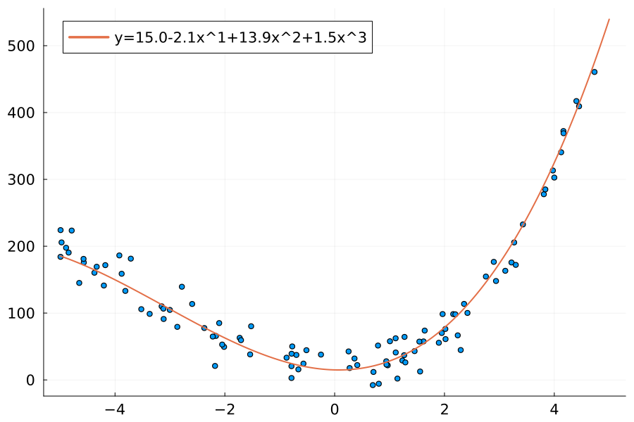
Gradient descent is a great algorithm to illustrate the usefulness of the code developed so far. The toy example of fitting a polynomial to data will be used. This is a useful example because (1) we can start with a target curve and so have ground truth values to compare and (2) this problem can be solved analytically without gradients.

Here is code to create the above data:
using StatsBase
target_weights = [15.0, -2.1, 13.9, 1.5]
noise_factor = 0.2
xs = (rand(100) .- 0.5) .* 10
ys = map(x -> evalpoly(x, target_weights), xs)
scale_factor = mean(abs.(ys))
ys .+= randn(length(ys)) * scale_factor * noise_factor
Analytical least squares fitting of polynomials ⇩
For a polynomial of order $p$, if there are exactly $n=p+1$ training samples (including for the constant $a_0$) than there exactly $n$ equations for $n$ unknowns ($a_0$,...,$a_p$) and this can be solved as an ordinary linear system: $$ \begin{align} &a_0 + a_1 x_1 + a_2x_1^2 + ... + a_p x_1^p = y_1 \\ &\vdots \\ &a_0 + a_1 x_n + a_2x_n^2 + ... + a_p x_n^p = y_n \\ &\Rightarrow \begin{bmatrix} 1 & x_1 & x_1^2 & \cdots & x_1^p \\ \vdots & \vdots & \vdots & \ddots & \vdots \\ 1 & x_n & x_n^2 & \cdots & x_n^p \end{bmatrix} \begin{bmatrix} a_0 \\ \vdots \\ a_n \end{bmatrix} = \begin{bmatrix} y_1 \\ \vdots \\ y_n \end{bmatrix} \\ &\Rightarrow XA=Y \\ &\Rightarrow A = X^{-1}Y \end{align} $$ Where $X^{-1}$ usually exists because $X$ is a square matrix.
However usually $n > p + 1$ and thus $X^{-1}$ will not exist. In that case the pseudoinverse $X^+$, also called the Moore-Penrose inverse, can be used instead: $$ \begin{align} X^{+} &= (X^T X)^{-1} X^T \\ \Rightarrow A &= X^{+}Y \end{align} $$ It can be proven that this solution for $A$ minimises the least squared error.
Here is this solution in code:
using LinearAlgebra
function solve_poly_linear(order::Int, xs::AbstractVector, ys::AbstractVector)
    n = length(xs)
    X = zeros(n, order + 1)
    for (i, x) in enumerate(xs)
        xpow = 1
        for j in 1:(size(X, 2))
            X[i, j] = xpow
            xpow *= x
        end
    end
    pinv(X) * ys
end
Here is a simple version of gradient descent:
Gradient descent
while (criteria is not met) do:
$\quad$ $\Delta = 0$
$\quad$ for sample, label in train_set do:
$\quad\quad$ $\Delta \leftarrow \Delta + \frac{\partial}{\partial\theta_j}L$($m_{\theta_j}$(sample), label)
$\quad$ $\theta_{j+1}$ $\leftarrow \theta_j - \alpha \Delta$
where $m_\theta$ is the model with parameters $\theta$ and $L$ is the loss function.
This is a Julia implementation for specifically applying the algorithm to polynomials.
The stopping condition is a maximum number of iterations, so the while loop has been replaced with a for loop.
The code also saves the loss so that the training progress can be analysed.
function gradient_descent_poly!(
    coeffs::AbstractVector,
    xs::AbstractVector,
    ys::AbstractVector
    ; learning_rate::AbstractFloat=0.1,
    max_iters::Integer=100
    )
    history = Float64[]
    n = length(xs)
    p = length(coeffs)
    for i in 1:max_iters
        loss_iter = 0.0
        Δcoeffs = zeros(p)
        for (x, y) in zip(xs, ys)
            # forward
            ŷ, back_poly = rrule(evalpoly, x, coeffs)
            loss_x, back_loss = rrule(mse, ŷ, y, n)
            # reverse
            Δloss, Δŷ, Δy, Δn = back_loss(1.0)
            Δevalpoly, Δx, Δcoeffs_x = back_poly(Δŷ)
            # accumulate
            loss_iter += loss_x
            Δcoeffs += Δcoeffs_x
        end
        # update
        coeffs .-= learning_rate .* Δcoeffs
        # history
        push!(history, loss_iter)
    end
    history
end
Calling the code:
coeffs = rand(4)
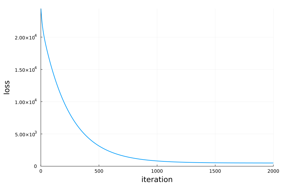
history = gradient_descent_poly!(coeffs, xs, ys; learning_rate=1e-5, max_iters=2000)
Plotting the history:

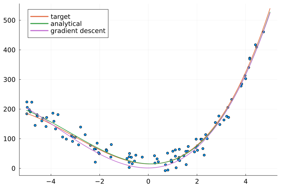
Comparing losses on the train set:
ys_est =  map(x -> evalpoly(x, coeffs), xs)
mse(ys_est, ys)| Method | Loss | Coefficients |
|---|---|---|
| Target | 416.62 | (15.0, -2.1, 13.9, 13.9, 1.5) |
| Analytical | 391.64 | (15.34, -3.24, 13.84, 1.46) |
| Gradient Descent | 498.50 | (1.37, 0.54, 14.51, 1.26) |
And finally, comparing the curves:
x_model = -5:0.01:5
ys_model =  map(x -> evalpoly(x, coeffs), x_model)
4.2 Revisited with map
It is possible to replace the inner loop over the training data with map.
function gradient_descent_poly!(
    coeffs::AbstractVector,
    xs::AbstractVector,
    ys::AbstractVector
    ; learning_rate::AbstractFloat=0.1,
    max_iters::Integer=100
    )
    history = Float64[]
    for i in 1:max_iters
        # forward
        ys_and_backs = map(x->rrule(evalpoly, x, coeffs), xs)
        ŷ = map(first, ys_and_backs)
        loss_iter, back_loss = rrule(mse, ŷ, ys)
        # reverse
        Δmse, Δŷ, Δy = back_loss(1.0)
        ∂f_and_∂x_zipped = map(((_, pb), δ) -> pb(δ), ys_and_backs, Δŷ)
        Δcoeffs_unzipped = map(Δ->Δ[3], ∂f_and_∂x_zipped) # Δ[i] = (Δevalpoly, Δx, Δcoeffs)
        Δcoeffs = reduce(+, Δcoeffs_unzipped)
        # update
        coeffs .-= learning_rate .* Δcoeffs
        # history
        push!(history, loss_iter)
    end
    history
end
This is code is slightly more complex than the previous version. The behaviour and performance is practically identical. However, it is one step closer to being more generic.
In machine learning, models usually execute on multiple inputs at once. We could make a polynomial model that does that:
struct Polynomial{V<:AbstractVector}
    weights::V
end
(m::Polynomial)(x) = evalpoly(x, m.weights)
(m::Polynomial)(x::AbstractVector) = map(m, x)
The goal then is to get gradients for the model’s weights directly:
model = Polynomial(coeffs)
zs, back = pullback(m -> m(xs), model)
In the next sections we will write code that will inspect the model function call, recognise that it calls map, and call a pullback for map.2
This in turn will call the pullback for evalpoly, which will pass the arguments to the rrule defined above.
5 Conclusion
The next two sections will develop the pullback function.
It will inspect and decompose code with the goal of passing arguments to rrule and accumulating gradients via the chain rule.
Part 2 will introduce metaprogamming Julia and generate expressions for the backpropagation code. However the code is unstable and prone to errors - it is recursive metaprogramming - so part 3 will introduce more robust code making use of the IRTools.jl package. This code really pushes Julia’s metaprogramming to its limits.
It is possible to jump straight to part 3 if desired.
-
For example, Micrograd defines a
Valueclass that has a custom definition for__add__. This custom definition then calculates the forward pass and prepares the backwards pass. The same is true of theTensorobjects in PyTorch. ↩ -
It is a design choice to use
pullbackand notrrulefor map. Bothrruleandpullbackhave the same outputs. Howeverrruleis intended for stand alone gradients, whereaspullbackwill potentially involve recursive calls to itself. ↩