Denoising diffusion probabilistic models from first principles

Denoising diffusion probabilistic models for AI art generation from first principles in Julia. This is part 1 of a 3 part series on these models.

Update 28 August 2023: code refactoring and update to Flux 0.13.11 explicit syntax.

This is part of a series. The other articles are:

• Part 2: image generation with MNIST.
• Part 3: classifier free guidance.

Full code available at github.com/LiorSinai/DenoisingDiffusion.jl. Examples notebooks at github.com/LiorSinai/DenoisingDiffusion-examples

Table of Contents

Introduction

It’s nearing the end of 2022 and one thing this year will be remembered for, for better or worse, is the breakthroughs in text to image generation. It very quickly went from a niche research topic to gathering excitement on tech websites to ethical debates on mainstream media. While people were asking what is it good for and others were making fun of nightmarish images by early prototypes AI generated art started flooding online art communities, artists debated their futures, savvy developers experimented with custom Photoshop plugins and it won art competitions. Companies have had to respond officially, whether it be Deviant Art’s DreamUp or Adobe’s new AI tools for Photoshop.

Google got people talking with their impressive Imagen text to image model but it was OpenAI’s beta rollout for DALLE 2 that opened it up to the world, giving people a chance to experiment with this new technology for the first time. Then came Midjourney offering an impressive model for a small monthly subscription fee. Then Stable Diffusion came and made everyone’s draw drop by offering everything - the model included - for free. Anyone with the equivalent of a high-end gaming computer and 10GB of video RAM could download it and run it themselves. While these requirements are steep for the average person, it is a very low bar for a model that compresses huge amounts of human creativity into a tiny digital space and that can create art beyond the ability of most people (except for trained artists of course).

The digital art landscape has materially shifted. It bears a resemblance to earlier creative technology revolutions such as changes to painting brought about by cameras and changes to music brought about by synthesizers. Like these previous revolutions it has not made artists or old techniques obsolete but it has shifted expectations and brought about new forms of creative work. How this impacts the world remains to be seen.

For the rest of this blog post however we’ll set aside these weighty philosophical questions and instead focus on the question, how is this possible?

Goals

A text to image model is made up of several models: a language model to convert words to vector embeddings, an image generation model to convert embeddings to images and a super-resolution network to upscale low resolution images. The last model is necessary because the image generation is expensive and it is much quicker to do on low resolution images. This series is limited to only the image generation model. The main goals are to explain how they work from first principles and to implement a full working model.

I’ll be using the MNIST dataset - a classic in machine learning - and eventually work up to the guided diffusion responsible for the video at the top. However part 1 will be on a much simpler problem: diffusing points to create a 2D spiral. This is a toy problem in the sense that it can be solved mathematically. In fact we’ll be using these mathematical techniques to assess our solution in the section Optimal solutions.

Many blog posts on this topic dive straight into the harder problem of image generation, such as this post by Assembly AI. I think this is a mistake as the model itself is as complex, if not more so, than all the mathematics behind diffusion. By starting off with the spiral we can use a much simpler model and focus more on the mathematics. It is also simpler and faster to test the code.

I’ll be using my favourite programming language, Julia. It is very well suited to the task because it is fast and comes with much of the needed functionality built in. As a partially typed language it is easy to interpret function calls, for both the coder and the compiler. That said, I found only one other DDPM repository in Julia (see here). It was a useful starting point but overall I found the code quality lacking.¹ Instead I mainly tried to emulate PyTorch code - this repository in particular.

Denoising diffusion probabilistic models

Image generation has been around for several years. The first models used variational autoencoders (VAEs) or generative adversarial networks (GANs). The big breakthrough over the past two years has been to use denoising diffusion probabilistic models (DDPMs) instead. DDPMs are more stable and so are easier to train than GANs and they generalise better than VAEs.

DDPMs were first introduced in the 2015 paper Deep Unsupervised Learning using Nonequilibrium Thermodynamics by Sohl-Dickstein et. al.. They tested their ideas on toy datasets like the spiral as well as on the CIFAR-10 image dataset. But their results were not state of the art. Instead it was the 2020 paper Denoising Diffusion Probabilistic Models by Jonathan Ho, Ajay Jain and Pieter Abbeel from Google Brain that really made an impact. This paper took the original ideas and applied several simplifications which made working with them easier. At the same time they used newer, bigger, more complex deep learning architectures, and hence were able to get state of the art high quality image generation.

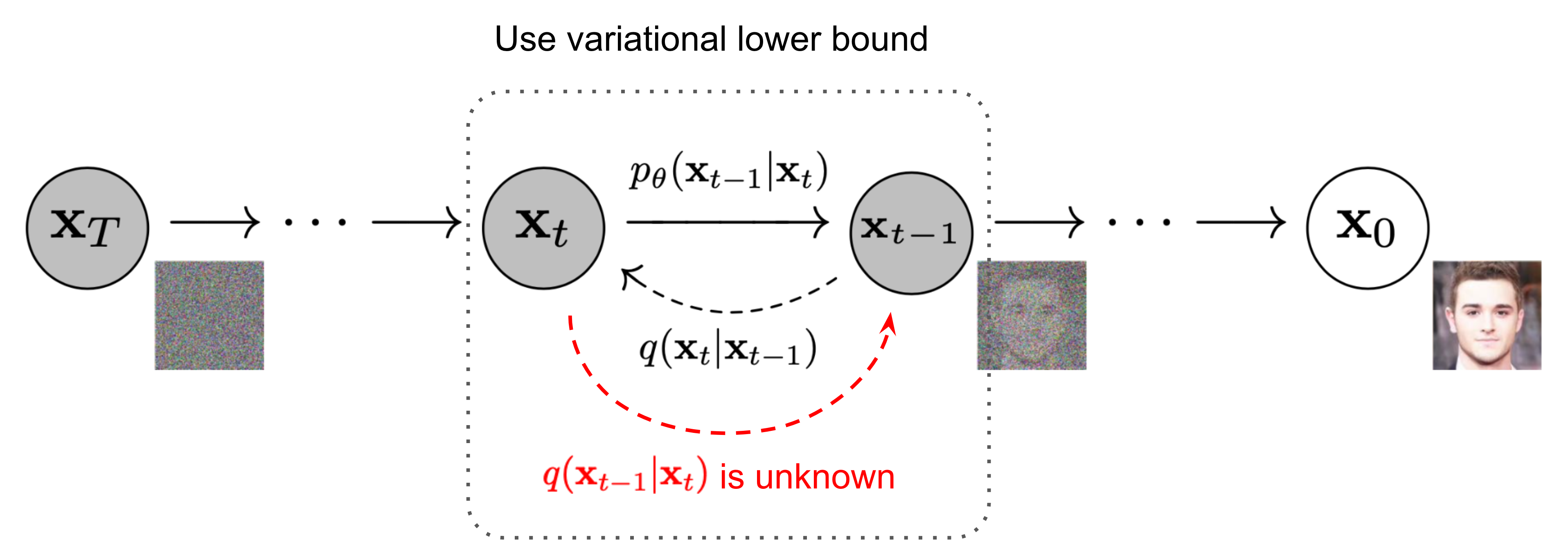
Denoising diffusion consists of two processes: a forward process which gradually adds noise to an image (right to left in the image above) and a reverse process which gradually removes noise (left to right). The forward process is denoted $q(x_t \vert x_{t-1})$.² It is done with a fixed stochastic process. In particular, Gaussian noise is gradually added to the image. The reverse process is $p_\theta(x_{t-1} \vert x_{t})$. This is the process that is parameterised and learnt. At sampling time a random noise is passed and the reverse process denoises it to form a new image.

The reason for using multiple time steps is to make the problem tractable. By analogy, it is difficult for a person to complete a painting in a single brush stroke. But an artist can create incredibly detailed works of art with many small brush strokes. In a similar way there is a big gap between a noisy and a clear image and it is difficult for a model to bridge it in one time step. By spreading the work over many time steps we can slowly reduce the noise and draw a final image.

The two source papers are both very accessible and are the main source material for this post. As a secondary source this blog post provides a succinct mathematical summary.

Preliminaries

Normal distribution

Theory

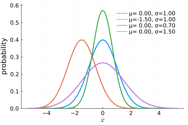
The normal distribution, also known as the Gaussian distribution, forms the basis of the diffusion model. Examples of it are shown above. This bell curve distribution arises naturally in nature. It also has nice mathematical properties.

The probability distribution function (pdf) is given by the following equation:

Where $\mu$ is the mean and $\sigma$ is the standard deviation.

The following notation is used to indicate that a sample $x$ is drawn from this distribution:

I prefer the first line but the second is what you’ll see in the papers.

We can simulate samples from any normal distribution by sampling from a $\mathcal{N}(0, 1)$ distribution and scaling and shifting:

Code

In code:

x = μ + σ * randn()

A full simulation:

using Plots, StatsBase
μ, σ, n = 1.5, 0.7, 1000
x = μ .+ σ .* randn(n);
h = fit(Histogram, x, nbins=50);
width = h.edges[1][2] - h.edges[1][1]
y = h.weights / sum(h.weights * width) ;
bar(h.edges[1], y, label="simulated", xlabel=L"x", ylabel="probability")

pdf(x, μ, σ) = 1/(σ * sqrt(2π)) * exp(-0.5 * (x - μ)^2/σ^2)
xt = -1:0.01:4
yt = pdf.(xt, μ, σ)
plot!(xt, yt, linewidth=3, label="theoretical")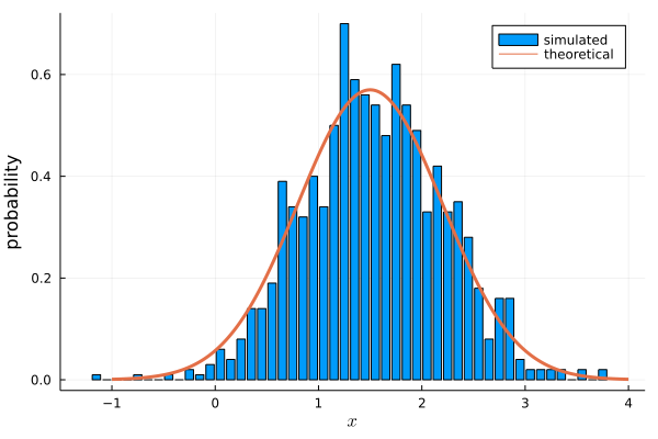

The inbuilt Julia function matches theory very well. If n is increased it works even better.

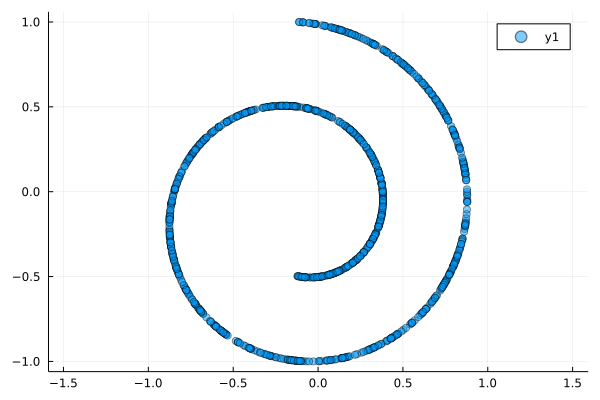
Spiral dataset

The following code is used to make the spiral based on Scikit-learn’s swiss roll code.

using Random
function make_spiral(rng::AbstractRNG, n_samples::Int=1000)
    t_min = 1.5π
    t_max = 4.5π

    t = rand(rng, n_samples) * (t_max - t_min) .+ t_min

    x = t .* cos.(t)
    y = t .* sin.(t)

    permutedims([x y], (2, 1))
end

make_spiral(n_samples::Int=1000) = make_spiral(Random.GLOBAL_RNG, n_samples)

Everything is normalised to lie between $-1$ and $1$:

function normalize_zero_to_one(x)
    x_min, x_max = extrema(x)
    x_norm = (x .- x_min) ./ (x_max - x_min)
    x_norm
end

function normalize_neg_one_to_one(x)
    2 * normalize_zero_to_one(x) .- 1
end

Plotting:

using Plots
n_samples = 1000
X = normalize_neg_one_to_one(make_spiral(n_samples))
scatter(X[1, :], X[2, :], 
    alpha=0.5,
    aspectratio=:equal,
    )

Implementation

Project setup

To start, make a package in the Julia REPL:

The purpose of making a package is that we can now use the super helpful Revise package, which will dynamically update most changes during development without errors:

julia> using Revise
julia> using DenoisingDiffusion

To follow this tutorial, it is recommended to load the dependencies directly:

using Flux
using NNlib
using BSON
using Printf
using ProgressMeter
using Random

You can see my final code at github.com/LiorSinai/DenoisingDiffusion.jl.

Forward process

Theory

The forward process takes this spiral and gradually adds noise until it is indistinguishable from Gaussian noise. It is a fixed Markov chain that adds Gaussian noise according to the schedule $\beta_1, \beta_2, …, \beta_T$ over $T$ time steps.

The $\beta$’s are chosen to be linearly increasing. These formulas then result in the variance increasing over time while the drift from the starting image decreases. (I can’t give a better reason for them).

Code

The $\beta$’s have to be manually tuned, so as a starting point we’ll use some existing values and scale accordingly:

function linear_beta_schedule(num_timesteps::Int, β_start=0.0001f0, β_end=0.02f0)
    scale = convert(typeof(β_start), 1000 / num_timesteps)
    β_start *= scale
    β_end *= scale
    range(β_start, β_end; length=num_timesteps)
end

Now create the schedule. I’ve manually tuned the starting and end $\beta$ values so the noising process happens evenly over the whole time range.

num_timesteps = 40
βs = linear_beta_schedule(num_timesteps, 8e-6, 9e-5)

And have a look at the results:³

Xt = X
anim = @animate for t ∈ 1:(num_timesteps + 10)
    if t < num_timesteps
        μ = Xt .* sqrt(1 - βs[t])
        noise = randn((2, size(X, 2)))
        σ = sqrt(βs[t]) 
        global Xt = μ + σ .* noise
    else
        Xt = Xt
        t = num_timesteps
    end
    p = scatter(Xt[1, :], Xt[2, :], alpha=0.5, label="", 
        aspectratio=:equal,
        xlims = (-2, 2), ylims=(-2, 2),
        title="t=$t"
    )
end

That was easy enough. The hard part is going to be starting with noise and reversing this process. (And not just by reversing the GIF!)

Shortcut

Theory

The above formula for $q(x_t | x_{t-1})$ requires iterating through all timesteps to get the result at $X_T$. However a nice property of the normal distribution is we can skip straight to any time step from the first time step $t=0$.

Define $\alpha_t = 1 - \beta_t$:

where $\bar{\alpha}_t = \prod_i^t \alpha_i=\prod_i^t (1-\beta_i)$. Line 5 uses the formula for the addition of two normal distributions:

More detail can be found here.

We now have a formula for $q(x_t \vert x_0)$:

Code

As an early optimisation we’ll pre-calculate all the $\beta$, $\alpha$ and $\bar{\alpha}$ values and store them in a struct. First create a GaussianDiffusion struct (more will be added to this struct later):

import Base.eltype

struct GaussianDiffusion{V<:AbstractVector}
    num_timesteps::Int
    data_shape::NTuple
    denoise_fn

    βs::V
    αs::V
    α_cumprods::V
    α_cumprod_prevs::V

    sqrt_α_cumprods::V
    sqrt_one_minus_α_cumprods::V
end

eltype(::Type{<:GaussianDiffusion{V}}) where {V} = V

function GaussianDiffusion(V::DataType, βs::AbstractVector, data_shape::NTuple, denoise_fn)
    αs = 1 .- βs
    α_cumprods = cumprod(αs)
    α_cumprod_prevs = [1, (α_cumprods[1:end-1])...]

    sqrt_α_cumprods = sqrt.(α_cumprods)
    sqrt_one_minus_α_cumprods = sqrt.(1 .- α_cumprods)

    GaussianDiffusion{V}(
        length(βs),
        data_shape,
        denoise_fn,
        βs,
        αs,
        α_cumprods,
        α_cumprod_prevs,
        sqrt_α_cumprods,
        sqrt_one_minus_α_cumprods,
    )
end

Define a helper extract function for broadcasting across batches. This will be needed later when training with multiple batches simultaneously.

function _extract(input, idxs::AbstractVector{Int}, shape::NTuple)
    reshape(input[idxs], (repeat([1], length(shape) - 1)..., :))
end

Next the q_sample function. The first method is the main definition. The other two are convenience functions so we can pass in time steps as a vector or integer without worrying about the noise. These other methods however need to be told where to place the noise: on the CPU or the GPU. If the model is on the GPU - as is commonly done with larger models - then all the data that is created also needs to be on the GPU. The Flux methods cpu and gpu are used for this through the to_device option. By default, to_device=cpu.

using Flux

function q_sample(
    diffusion::GaussianDiffusion, x_start::AbstractArray,
    timesteps::AbstractVector{Int}, noise::AbstractArray
    )
    coeff1 = _extract(diffusion.sqrt_α_cumprods, timesteps, size(x_start))
    coeff2 = _extract(diffusion.sqrt_one_minus_α_cumprods, timesteps, size(x_start))
    coeff1 .* x_start + coeff2 .* noise
end

function q_sample(
    diffusion::GaussianDiffusion, x_start::AbstractArray,
    timesteps::AbstractVector{Int}
    ; to_device=cpu
    )
    T = eltype(eltype(diffusion))
    noise =  randn(T, size(x_start)) |> to_device
    timesteps = timesteps |> to_device
    q_sample(diffusion, x_start, timesteps, noise)
end

function q_sample(
    diffusion::GaussianDiffusion, x_start::AbstractArray{T, N}, timestep::Int
    ; to_device=cpu
    ) where {T, N}
    timesteps = fill(timestep, size(x_start, N)) |> to_device
    q_sample(diffusion, x_start, timesteps; to_device=to_device)
end

Testing it out:

num_timesteps = 40
βs = linear_beta_schedule(num_timesteps, 8e-6, 9e-5)
diffusion = GaussianDiffusion(Vector{Float32}, βs, (2,), identity)
canvases = []
for frac in [0.0, 0.25, 0.5, 0.75, 1]
    local p
    timestep = max(1, ceil(Int, frac * num_timesteps))
    Xt = q_sample(diffusion, X, timestep)
    p = scatter(Xt[1, :], Xt[2, :], alpha=0.5, label="", 
        aspectratio=:equal,
        xlims = (-2, 2), ylims=(-2, 2),
        title="t=$timestep"
        )
    push!(canvases, p)
end

The result:

Reverse process

Theory

Now to calculate the reverse process $p_\theta(x_{t-1} | x_{t})$. The trick here is that while we do not have a direct expression for $p_\theta(x_{t-1} | x_{t})$, we can calculate an expression for the posterior probability $q(x_{t-1} | x_{t}, x_0)$ using Bayes’ theroem. This is the red arrow in the original denoising image. That is, given the current time step and the start image, we can with a high probability deduce what the previous time step was based on the known probability distributions. Of course this statement is nonsensical in that we don’t have the start image - if we did we wouldn’t need to go through this process. However what we can do is use a model to predict a start image and refine it at every time step. The analogy I used earlier therefore needs correcting: while we can’t jump straight from noise to a good starting image, we can estimate a bad start image and refine it.

Given our start image estimate $\hat{x}_0$, we can calculate the reverse process as:

where the second line expresses Bayes’ Theorem.

It is now a matter of substituting in equations $\eqref{eq:normal}$, $\eqref{eq:forward}$ and $\eqref{eq:shortcut-normal}$ and simplifying. The algebra however is somewhat lengthy.

Full derivation ⇩

The result is that $x_{t-1}$ is also a normal distribution $x_{t-1} \sim \mathcal{N}(\tilde{\mu}_t, \tilde{\beta}_t) $:

From the derivation the posterior mean $\tilde{\mu}_t$ and posterior standard deviation $\tilde{\beta}_t$ are:

Furthermore, Ho et al. show that we can use the shortcut formula $\eqref{eq:shortcut}$ for this $\hat{x}_0$:

The only free variable here is $\bar{z}$, the noise. This is the only value we’ll need to predict with the model: $\bar{z}=\epsilon_\theta(x_t, t)$. Rather than predicting the starting image directly, we will predict the noise that needs to be removed at each time step to get to it.

We can substitute equation $\eqref{eq:x0_estimate}$ into $\eqref{eq:posterior}$, but this form is not very useful because we will want to retrieve our estimates as well (for example the top image):

To recap:

1. We could predict $p_\theta(x_{t-1} \vert x_{t})$ directly but it is better to use an analytical expression requiring $\tilde{\mu}_t$ and $\tilde{\beta}_t$ $\eqref{eq:reverse}$.
2. We could predict $\tilde{\mu}_t$ directly but it is better to use an analytical expression requiring $x_t$ and $\hat{x}_0$ $\eqref{eq:posterior}$.
3. We could predict $\hat{x}_0$ directly but it is better to use an an analytical expression requiring $\epsilon_\theta$ $\eqref{eq:x0_estimate}$.

Code

As before we’ll pre-calculate all the co-efficients in the preceding equations.

import Base.eltype

struct GaussianDiffusion{V<:AbstractVector}
    num_timesteps::Int
    data_shape::NTuple
    denoise_fn

    βs::V
    αs::V
    α_cumprods::V
    α_cumprod_prevs::V

    sqrt_α_cumprods::V
    sqrt_one_minus_α_cumprods::V
    sqrt_recip_α_cumprods::V
    sqrt_recip_α_cumprods_minus_one::V
    posterior_variance::V
    posterior_log_variance_clipped::V
    posterior_mean_coef1::V
    posterior_mean_coef2::V
end

eltype(::Type{<:GaussianDiffusion{V}}) where {V} = V

Flux.@functor GaussianDiffusion
Flux.trainable(g::GaussianDiffusion) = (; g.denoise_fn) # only the denoise_fn is trainable

function GaussianDiffusion(
    V::DataType, βs::AbstractVector, data_shape::NTuple, denoise_fn
    )
    αs = 1 .- βs
    α_cumprods = cumprod(αs)
    α_cumprod_prevs = [1, (α_cumprods[1:end-1])...]

    sqrt_α_cumprods = sqrt.(α_cumprods)
    sqrt_one_minus_α_cumprods = sqrt.(1 .- α_cumprods)
    sqrt_recip_α_cumprods = 1 ./ sqrt.(α_cumprods)
    sqrt_recip_α_cumprods_minus_one = sqrt.(1 ./ α_cumprods .- 1)

    posterior_variance = βs .* (1 .- α_cumprod_prevs) ./ (1 .- α_cumprods)
    posterior_log_variance_clipped = log.(max.(posterior_variance, 1e-20))

    posterior_mean_coef1 = βs .* sqrt.(α_cumprod_prevs) ./ (1 .- α_cumprods)
    posterior_mean_coef2 = (1 .- α_cumprod_prevs) .* sqrt.(αs) ./ (1 .- α_cumprods)

    GaussianDiffusion{V}(
        length(βs),
        data_shape,
        denoise_fn,
        βs,
        αs,
        α_cumprods,
        α_cumprod_prevs,
        sqrt_α_cumprods,
        sqrt_one_minus_α_cumprods,
        sqrt_recip_α_cumprods,
        sqrt_recip_α_cumprods_minus_one,
        posterior_variance,
        posterior_log_variance_clipped,
        posterior_mean_coef1,
        posterior_mean_coef2
    )
end

First is equation $\eqref{eq:x0_estimate}$ for $\hat{x}_0$:

function predict_start_from_noise(
    diffusion::GaussianDiffusion, x_t::AbstractArray,
    timesteps::AbstractVector{Int}, noise::AbstractArray
    )
    coeff1 = _extract(diffusion.sqrt_recip_α_cumprods, timesteps, size(x_t))
    coeff2 = _extract(diffusion.sqrt_recip_α_cumprods_minus_one, timesteps, size(x_t))
    coeff1 .* x_t - coeff2 .* noise
end

function denoise(
    diffusion::GaussianDiffusion, x::AbstractArray,
    timesteps::AbstractVector{Int}
    )
    noise = diffusion.denoise_fn(x, timesteps)
    x_start = predict_start_from_noise(diffusion, x, timesteps, noise)
    x_start, noise
end

Then we can now use $\hat{x}_0$ in equation $\eqref{eq:posterior}$ for $\tilde{\mu}_t$ and $\tilde{\beta}_t$:

function q_posterior_mean_variance(
    diffusion::GaussianDiffusion, x_start::AbstractArray, x_t::AbstractArray,
    timesteps::AbstractVector{Int}
    )
    coeff1 = _extract(diffusion.posterior_mean_coef1, timesteps, size(x_t))
    coeff2 = _extract(diffusion.posterior_mean_coef2, timesteps, size(x_t))
    posterior_mean = coeff1 .* x_start + coeff2 .* x_t
    posterior_variance = _extract(diffusion.posterior_variance, timesteps, size(x_t))
    posterior_mean, posterior_variance
end 

And finally equation $\eqref{eq:reverse}$ for the reverse process for $x_{t-1}$, additionally returning $\hat{x}_0$:

function p_sample(
    diffusion::GaussianDiffusion, x::AbstractArray,
    timesteps::AbstractVector{Int}, noise::AbstractArray
    ; clip_denoised::Bool=true, add_noise::Bool=true
    )
    x_start, pred_noise = denoise(diffusion, x, timesteps)
    if clip_denoised
        clamp!(x_start, -1, 1)
    end
    posterior_mean, posterior_variance = q_posterior_mean_variance(
        diffusion, x_start, x, timesteps
    )
    x_prev = posterior_mean
    if add_noise
        x_prev += sqrt.(posterior_variance) .* noise
    end
    x_prev, x_start
end

The option for clip_denoised is just to improve results and is not part of the analytical equations. The option for add_noise should always be true except for the timestep of $t=0$.

We don’t have a model yet, but for now we can test these functions with a very bad denoise_fn that simply returns a random matrix:

diffusion = GaussianDiffusion(Vector{Float32}, βs, (2,), (x, t) -> randn(size(x)))
XT = randn((2, 100))
timesteps = fill(num_timesteps, 100)

x_start, pred_noise = DenoisingDiffusion.denoise(diffusion, XT, timesteps)
posterior_mean, posterior_variance = q_posterior_mean_variance(diffusion, x_start, XT, timesteps)
noise =  randn(size(XT))
x_prev = posterior_mean + sqrt.(posterior_variance) .* noise

Full loop

Let’s create a full loop through the reverse process:

using Flux, ProgressMeter
function p_sample_loop(
    diffusion::GaussianDiffusion, shape::NTuple
    ; clip_denoised::Bool=true, to_device=cpu
    )
    T = eltype(eltype(diffusion))
    x = randn(T, shape) |> to_device
    @showprogress "Sampling..." for t in diffusion.num_timesteps:-1:1
        timesteps = fill(t, shape[end]) |> to_device;
        noise =  randn(T, size(x)) |> to_device
        x, x_start = p_sample(
            diffusion, x, timesteps, noise
            ; clip_denoised=clip_denoised, add_noise=(t != 1)
        )
    end
    x
end

function p_sample_loop(diffusion::GaussianDiffusion, batch_size::Int; options...)
    p_sample_loop(diffusion, (diffusion.data_shape..., batch_size); options...)
end

We can test it with:

diffusion = GaussianDiffusion(Vector{Float32}, βs, (2,), (x, t) -> randn(size(x)))
X0 = p_sample_loop(diffusion, 100, clip_denoised=false)

It works but if you plot it, you’ll just get random noise. X0 is no closer to a spiral than XT. We need a much better denoise_fn than random noise.

This function only returns the last image. For making time lapses we also want a loop which returns all images. If we were using an interpreted language like Python it might be acceptable to add an option to the p_sample function for this. Julia however is a compiled language and because the returned type is different it is better to have a separate function to preserve type safety:

function p_sample_loop_all(
    diffusion::GaussianDiffusion, shape::NTuple
    ; clip_denoised::Bool=true, to_device=cpu
    )
    T = eltype(eltype(diffusion))
    x = randn(T, shape) |> to_device
    x_all = Array{T}(undef, size(x)..., 0) |> to_device
    x_start_all = Array{T}(undef, size(x)..., 0) |> to_device
    tdim = ndims(x_all)
    @showprogress "Sampling..." for t in diffusion.num_timesteps:-1:1
        timesteps = fill(t, shape[end]) |> to_device;
        noise =  randn(T, size(x)) |> to_device
        x, x_start = p_sample(
            diffusion, x, timesteps, noise
            ; clip_denoised=clip_denoised, add_noise=(t!= 1)
        )
        x_all = cat(x_all, x, dims=tdim)
        x_start_all = cat(x_start_all, x_start, dims=tdim)
    end
    x_all, x_start_all
end

function p_sample_loop_all(diffusion::GaussianDiffusion, batch_size::Int=16; options...)
    p_sample_loop_all(diffusion, (diffusion.data_shape..., batch_size); options...)
end

Model

When I first tried this problem I struggled to build a sufficiently good enough model. Sohl-Dickstein et al. used a radial basis function. However my implementation didn’t perform well. It is this blog post that I owe to breaking my impasse.⁴

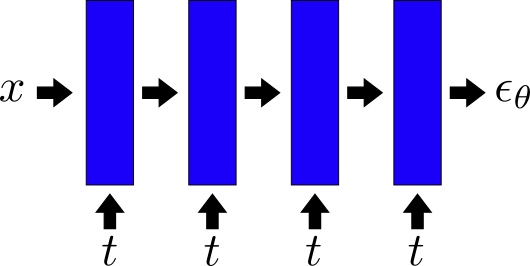
The important observation is that the model is time dependent. It takes in two inputs, $x$ and $t$, and it must satisfy two seemingly conflicting requirements: (1) its weights must be time dependent but also (2) they should be shared across time for efficiency. To achieve this the Sohl-Dickstein et al. model had some independent layers per time step and some shared layers. A much simpler approach is to use embedding vectors and add these to the outputs of each layer. This is known as “conditioning” the outputs.

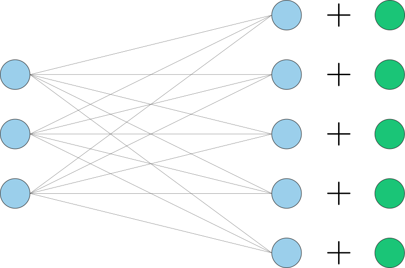
Using the Flux machine library we can build each layer with existing inbuilt functions:

Parallel(.+, Dense(d_in, d_out), Embedding(num_timesteps, d_out))

Flux also comes with the flexible Flux.Chain for building models. It only works for one input, but it is very easy to create an extension which works for multiple inputs based off the source code:

Imports:

using Flux
import Flux._show_children
import Flux._big_show

Definitions:

abstract type AbstractParallel end

_maybe_forward(layer::AbstractParallel, x::AbstractArray, ys::AbstractArray...) = 
    layer(x, ys...)
_maybe_forward(layer::Parallel, x::AbstractArray, ys::AbstractArray...) = 
    layer(x, ys...)
_maybe_forward(layer, x::AbstractArray, ys::AbstractArray...) = 
    layer(x)

struct ConditionalChain{T<:Union{Tuple,NamedTuple}} <: AbstractParallel
    layers::T
end
Flux.@functor ConditionalChain 

ConditionalChain(xs...) = ConditionalChain(xs)
function ConditionalChain(; kw...)
  :layers in keys(kw) && throw(ArgumentError("a Chain cannot have a named layer called `layers`"))
  isempty(kw) && return ConditionalChain(())
  ConditionalChain(values(kw))
end

Flux.@forward ConditionalChain.layers Base.getindex, Base.length, Base.first, Base.last,
Base.iterate, Base.lastindex, Base.keys, Base.firstindex

Base.getindex(c::ConditionalChain, i::AbstractArray) = ConditionalChain(c.layers[i]...)

Forward pass:

function (c::ConditionalChain)(x, ys...) 
    for layer in c.layers
        x = _maybe_forward(layer, x, ys...)
    end
    x
end

Printing:

function Base.show(io::IO, c::ConditionalChain)
    print(io, "ConditionalChain(")
    Flux._show_layers(io, c.layers)
    print(io, ")")
end

function _big_show(io::IO, m::ConditionalChain{T}, indent::Int=0, name=nothing) where T <: NamedTuple
    println(io, " "^indent, isnothing(name) ? "" : "$name = ", "ConditionalChain(")
    for k in Base.keys(m.layers)
        _big_show(io, m.layers[k], indent+2, k)
    end
    if indent == 0  
        print(io, ") ")
        _big_finale(io, m)
      else
        println(io, " "^indent, ")", ",")
    end
end

function Base.show(io::IO, m::MIME"text/plain", x::ConditionalChain)
    if get(io, :typeinfo, nothing) === nothing  # e.g. top level in REPL
        Flux._big_show(io, x)
    elseif !get(io, :compact, false)  # e.g. printed inside a Vector, but not a Matrix
        Flux._layer_show(io, x)
    else
        show(io, x)
    end
end

Create our model (we could also use .* instead of .+ as the connector):

d_hid = 32
num_timesteps = 40
model = ConditionalChain(
    Parallel(.+, Dense(2, d_hid), Embedding(num_timesteps, d_hid)),
    swish,
    Parallel(.+, Dense(d_hid, d_hid), Embedding(num_timesteps, d_hid)),
    swish,
    Parallel(.+, Dense(d_hid, d_hid), Embedding(num_timesteps, d_hid)),
    swish,
    Dense(d_hid, 2),
)

The result:

ConditionalChain(
  Parallel(
    Base.Broadcast.BroadcastFunction(+),
    Dense(2 => 32),                     # 96 parameters
    Embedding(40 => 32),                # 1_280 parameters
  ),
  NNlib.swish,
  Parallel(
    Base.Broadcast.BroadcastFunction(+),
    Dense(32 => 32),                    # 1_056 parameters
    Embedding(40 => 32),                # 1_280 parameters
  ),
  NNlib.swish,
  Parallel(
    Base.Broadcast.BroadcastFunction(+),
    Dense(32 => 32),                    # 1_056 parameters
    Embedding(40 => 32),                # 1_280 parameters
  ),
  NNlib.swish,
  Dense(32 => 2),                       # 66 parameters
)                   # Total: 11 arrays, 6_114 parameters, 24.711 KiB.

Sinusodial embeddings

Using Flux.Embedding works sufficiently well. However I find results are better with sinusodial embeddings, an idea that was proposed for transformers in the 2017 paper Attention is all you need. For a full explanation please see an earlier post on transformers.

i

0

Left: heatmap of the sinusodial embedding. Right: Sine wave with discrete sampling points corresponding to odd numbered rows.

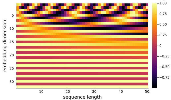
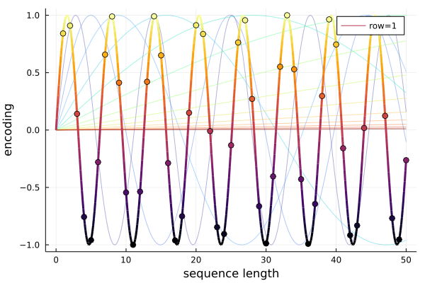
The short explanation is that we create a matrix where every column as a whole is unique. Each column can then be used as a time embedding for a particular time step. The uniqueness of each column is accomplished by using periodic trigonometric functions for the rows with gradually increasing frequency. See the above image for a visual demonstration.

The code is as follows:

struct SinusoidalPositionEmbedding{W<:AbstractArray}
    weight::W
end

Flux.@functor SinusoidalPositionEmbedding
Flux.trainable(emb::SinusoidalPositionEmbedding) = (;) # mark it as an non-trainable array

function SinusoidalPositionEmbedding(in::Int, out::Int)
    W = make_positional_embedding(out, in)
    SinusoidalPositionEmbedding(W)
end

function make_positional_embedding(dim_embedding::Int, seq_length::Int=1000; n::Int=10000)
    embedding = Matrix{Float32}(undef, dim_embedding, seq_length)
    for pos in 1:seq_length
        for row in 0:2:(dim_embedding-1)
            denom = 1.0 / (n^(row / (dim_embedding-2)))
            embedding[row + 1, pos] = sin(pos * denom)
            embedding[row + 2, pos] = cos(pos * denom)
        end
    end
    embedding
end

(m::SinusoidalPositionEmbedding)(x::Integer) = m.weight[:, x]
(m::SinusoidalPositionEmbedding)(x::AbstractVector) = NNlib.gather(m.weight, x)
(m::SinusoidalPositionEmbedding)(x::AbstractArray) = reshape(m(vec(x)), :, size(x)...)

function Base.show(io::IO, m::SinusoidalPositionEmbedding)
    print(io, "SinusoidalPositionEmbedding(", size(m.weight, 2), " => ", size(m.weight, 1), ")")
end

Used in a model:

model = ConditionalChain(
    Parallel(
        .+, 
        Dense(2, d_hid), 
        Chain(
            SinusoidalPositionEmbedding(num_timesteps, d_hid), 
            Dense(d_hid, d_hid))
        ),
    swish,
    Parallel(
        .+, 
        Dense(d_hid, d_hid), 
        Chain(
            SinusoidalPositionEmbedding(num_timesteps, d_hid), 
            Dense(d_hid, d_hid))
        ),
    swish,
    Parallel(
        .+, 
        Dense(d_hid, d_hid), 
        Chain(
            SinusoidalPositionEmbedding(num_timesteps, d_hid), 
            Dense(d_hid, d_hid))
        ),
    swish,
    Dense(d_hid, 2),
)

Training

Theory

We now need to train our model. We first need a loss function. We have two probability distributions, the forward process $q(x_{t}|x_{t-1})$ and the reverse process $p_\theta(x_{t-1} \vert x_{t})$ and ideally we would have a loss function that keeps them in sync. Put another way, if we start with $x_t$ and apply the forward process and then the reverse process, they should cancel each other out and return $x_t$.

We first start with an ideal loss function that minimises the error over the whole reconstruction process. This is the negative log likelihood:⁵

Sohl-Dickstein et. al. show that by substituting in equation $\ref{eq:bayes}$ this can be rewritten as:

The first term is the loss for the forward process but because this is fixed and has no parameters we can ignore it. The second term is called the “reconstruction error” and we can ignore it too because it only affects one time step. (The reconstruction error is more important for VAEs.) The last term is the KL divergence between two normal distributions which has a known formula. However Ho et. al. show that by substituting into that we can simplifier much further:

Where the expectation $\mathbb{E}$ is now simply an average. For more detail, please see the source papers or Lilian Weng’s post or Angus Turner’s post.

The end result is: since we are only predicting the noise $\epsilon_\theta$, we simply use the difference between the actual noise and the predicted noise as our loss function. Furthermore, we can consider each time step independently. So we can apply $\eqref{eq:shortcut}$ and take the difference between the model’s outputs and the $\bar{z}$ term. This is a weak signal and will require many training time steps, but it is incredibly simple to implement.

The next question is, how to implement the training loop? An obvious approach is to loop over every sample over very timestep and apply the above loss function. But once again Ho et. al. have a much simpler and more effective solution: to evenly distribute training, sample random time steps and apply the above loss function.

Training algorithm
repeat
$x_0 \sim q(x_0)$
$t \sim \text{Uniform}( \{ 1,\dots, T \} )$
$\epsilon \sim \mathcal{N}(0, \mathbf{I})$
$ x_t = \sqrt{\vphantom{1}\bar{\alpha}_t} x_0 + \sqrt{1 - \bar{\alpha}_t} \epsilon $
Take gradient descent step on
$\quad \nabla_\theta ||\epsilon - \epsilon_\theta||^2 $
until converged

Code

The code is slightly more generic in that you can pass any loss function to evaluate the difference. For example, Flux.mae or Flux.mse. The first method calculates the losses from all three inputs (x_start, timesteps and noise) while the second generates the timesteps and noise and then calls the first.

function p_losses(
    diffusion::GaussianDiffusion, loss, x_start::AbstractArray,
    timesteps::AbstractVector{Int}, noise::AbstractArray
    )
    x = q_sample(diffusion, x_start, timesteps, noise)
    model_out = diffusion.denoise_fn(x, timesteps)
    loss(model_out, noise)
end

function p_losses(
    diffusion::GaussianDiffusion, loss, x_start::AbstractArray{T, N}
    ; to_device=cpu
    ) where {T, N}
    timesteps = rand(1:diffusion.num_timesteps, size(x_start, N)) |> to_device
    noise = randn(eltype(eltype(diffusion)), size(x_start)) |> to_device
    p_losses(diffusion, loss, x_start, timesteps, noise)
end

This can be used with the inbuilt Flux.train! function. Here is also a custom function which additionally returns a training history and displays a progress bar. For more functionality like calculating the validation loss after each epoch, see the train.jl script in the repository.

using Flux: DataLoader
using ProgressMeter
using Printf

function train!(loss, model, data::DataLoader, opt_state;
    num_epochs::Int=10,
    )
    history = Dict("mean_batch_loss" => Float64[])
    for epoch = 1:num_epochs
        progress = Progress(length(data); desc="epoch $epoch/$num_epochs")
        total_loss = 0.0
        for (idx, x) in enumerate(data)
            batch_loss, grads = Flux.withgradient(model) do m
                loss(m, x)
            end
            total_loss += batch_loss
            Flux.update!(opt_state, model, grads[1])
            ProgressMeter.next!(progress)
        end
        push!(history["mean_batch_loss"], total_loss / length(data))
        @printf("mean batch loss: %.5f\n", history["mean_batch_loss"][end])
    end
    history
end

Results

At long last, we can implement the full training algorithm:

βs = linear_beta_schedule(num_timesteps, 8e-6, 9e-5)
diffusion = GaussianDiffusion(Vector{Float32}, βs, (2,), model)

diffusion = diffusion |> to_device

train_data = Flux.DataLoader(X |> to_device; batchsize=32, shuffle=true);
loss_type = Flux.mse;
loss(diffusion, x) = p_losses(diffusion, loss_type, x; to_device=to_device)
opt = Adam(0.001);
opt_state = Flux.setup(opt, diffusion)
history = train!(
    loss, diffusion, train_data, opt_state
    ; num_epochs=100
)

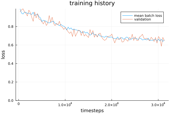
The training history:

Sampling and plotting:

Xs, X0s = p_sample_loop_all(diffusion, 1000) ;
anim_denoise = @animate for i ∈ 1:(num_timesteps + 10)
    i = i > num_timesteps ? num_timesteps : i
    p1 = scatter(Xs[1, :, i], Xs[2, :, i], 
        alpha=0.5, 
        title=L"${x}_t$", 
        label="",
        aspectratio=:equal,
        xlims=(-2, 2), ylims=(-2, 2),
        figsize=(400, 400),
    )
    p2= scatter(X0s[1, :, i], X0s[2, :, i], 
        alpha=0.5, 
        title=L"$\hat{x}_0$", 
        label="",
        aspectratio=:equal,
        xlims = (-2, 2), ylims=(-2, 2),
        figsize=(400, 400),
    )
    plot(p1, p2, plot_title="i=$i")
end
gif(anim_denoise, joinpath(directory, "reverse_x0.gif"), fps=8)

Evaluation

Optimal solutions

Theory

Given a random point in space:

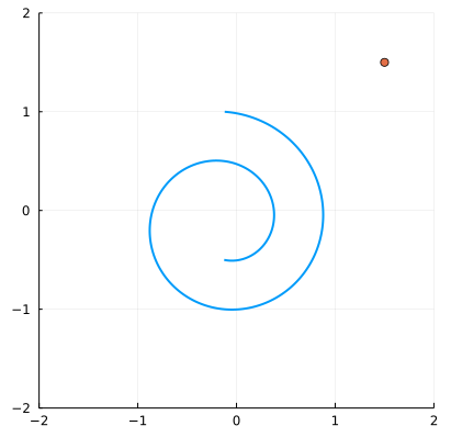
We can find the closest point on the spiral to it. It will lie along a line that is perpendicular to the tangent of the spiral:

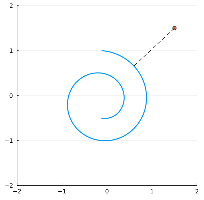
This gives us a natural way to evaluate how good our solution is: we want to minimise the sum (average) of our lines to the base spiral. This will therefore require a general formula for getting the shortest distance to the spiral.

The equation of the spiral is:

Where $1.5\pi \leq t \leq 4.5\pi$.

It is normalised by a scale factor of $s=\frac{2}{x_{max}-x_{min}}=\frac{1}{4\pi}$ and shifted by $c=-1 - sx_{min}=-\frac{1}{8}$. The normalised function is then:

The Euclidean distance from a point $p$ to the spiral is an application of Pythagorus:

Finding the closest point on the spiral is equivalent to minimising this equation with respect to $t$, which happens when the gradient is zero:

There is no analytical solution for $t$ in this equation. However we can solve it numerically easy enough. I’ll be using a custom implementation of Newton’s method but there are many other solvers in Julia. Or a brute force approach is good enough.

Code

First define the equations for the spiral:

θmin = 1.5π
θmax = 4.5π
xmax = 4.5π
xmin = -3.5π
x_func(t) = t * cos(t) 
y_func(t) = t * sin(t)

scale = 2/(xmax - xmin)
shift = -1 - scale * xmin
x_func_norm(t) = scale * x_func(t) + shift
y_func_norm(t) = scale * y_func(t) + shift

Next define the main equation and its deravitives. Newton’s method requires the devirative of the equation we are solving, which is the second derivative with respect to $D(p, t)$:

f(p, t)   = (x_func_norm(t) - p[1])^2 + (y_func_norm(t) - p[2])^2;
df(p, t)  = t * scale + (shift - p[1]) * (cos(t) - t * sin(t)) + (shift - p[2]) * (sin(t) + t * cos(t));
ddf(p, t) = scale - (shift - p[1]) * (2sin(t) + t * cos(t)) + (shift - p[2]) * (2cos(t) - t * sin(t));

Equation $\eqref{eq:opt}$ has multiple roots as a result of the periodic nature of the spiral. Every full revolution there is another candidate for the closest point to the spiral. Depending on the range we choose the answer will be different. Therefore in order for Newton’s method to converge to a good answer, we need to provide a good first guess.⁶ This is done by brute force: pass $n$ points in a range to the function and choose the one with the smallest outcome. As of Julia 1.7 this is inbuilt into the argmin function. (You could also only use this brute force method without Newton’s method because the extra precision provided is not critical.)

function argmin_func_newton(
    f, df, ddf, tmin::AbstractFloat, tmax::AbstractFloat; 
    num_iters::Int=10, length::Int=100
    )
    seed = argmin(f, range(tmin, tmax, length))
    root = newtons_method(df, ddf, seed, tmin, tmax; num_iters=num_iters)
    root
end

function newtons_method(
    f, fgrad, root::AbstractFloat, rmin::AbstractFloat, rmax::AbstractFloat
    ; num_iters::Int=10, ϵ::AbstractFloat=0.3
    )
    grad = fgrad(root)
    if (abs(grad) < ϵ) 
        @warn("gradient=$grad is too low for Newton's method. Returning seed without optimization.")
        return root
    end
    for i in 1:num_iters
        root = root - f(root)/fgrad(root)
        root = clamp(root, rmin, rmax)
    end
    root
end

Applying the solver:

solver(p) = argmin_func_newton(t->f(p, t), t->df(p, t), t->ddf(p, t), θmin, θmax)

closest_points = Matrix(undef, num_samples, num_timesteps);
closest_distances = Matrix(undef, num_samples, num_timesteps);

@time for timestep in 1:num_timesteps
    points = Xs[:, :, timestep]
    ts = [solver(points[:, i]) for i in 1:num_samples]
    ds = [f(points[:, i], ts[i]) for i in 1:num_samples]
    
    closest_points[:, timestep] .= ts
    closest_distances[:, timestep] .= sqrt.(ds)
end

Plotting the results:

canvases = []
max_samples = size(Xs, 2)
n = 200
for frac in [0.0, 0.25, 0.5, 0.75, 1.0]
    local p
    timestep = max(1, ceil(Int, frac * num_timesteps))
    p = plot(x, y, aspectratio=:equal, label="", linewidth=2, title="t=$timestep")
    points = Xs[:, :, timestep]    
    ts = closest_points[:, timestep]
    xt = x_func_norm.(ts)
    yt = y_func_norm.(ts)
    for i in 1:n
        plot!(p, [points[1, i] ;xt[i]], [points[2, i]; yt[i]], label="", color=:black )
    end
    push!(canvases, p)
end
plot(canvases..., layout=(1, 5), link=:both, size=(900, 200))

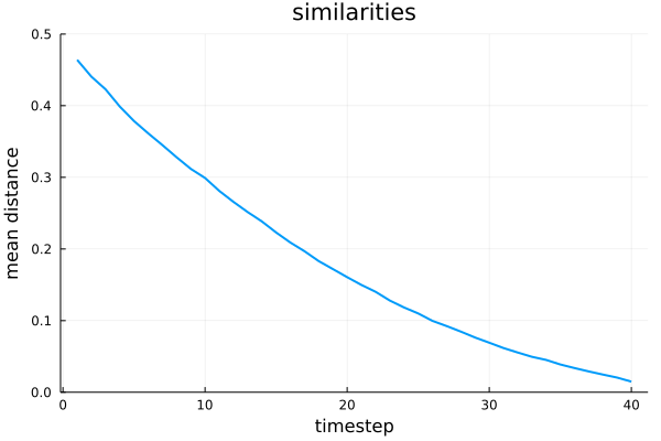
And finally, finding the average distance over time:

similarities = mean(closest_distances, dims=1)
@printf("Starting similarity: %.4f\n", similarities[1])
@printf("Final similarity:    %.4f\n", similarities[end])

p = plot(1:num_timesteps, vec(similarities),
    ylims=(0, 0.5),
    label="",
    xlabel="timestep",
    ylabel="mean distance",
    title="similarities",
    linewidth=2
)

As an added bonus, one can imagine denoising points by moving them along the line of shortest distance towards the spiral. This is the optimal denoising solution which moves the points the least to create the spiral. If we interpolate linearly over the whole time period such that that each points moves a fraction $\frac{1}{T}$ along this line at each time step $t$ we get this pleasing result:

Regretably we will not however be able to apply these optimal techniques to the harder problem of image generation. There is indeed no optimal solution for creativity.

Conclusion

This post has layed the groundwork for denoising diffusion probabilistic models. We’ll be able to reuse nearly all of the functions in this post for the next post on image generation. The only difference is we’ll be making a much more complex model for the denoise_fn. See part 2.

Something else you might want to try is working with patterns other than a spiral. What happens if you try train a model on multiple patterns at once? Part 3 will investigate this and provide a method to direct which pattern is produced. That same method is used with text embeddings to direct the outcome of AI art generators.

Appendix

Bayes’ theorem for normal distributions

This is a generalisation of the result proved in Reverse process. That proof only relied on algebra whereas this one relies on calculus too.

If a normal distribution $x_{x|y}\sim \mathcal{N}(cy, \sigma_{xy}^2)$ has a mean that is also normally distributed according to $y\sim \mathcal{N}(\mu_y, \sigma_y^2)$ for a constant $c$, then the conditional probability of $p(y \vert x)$ is also a normal distribution with $\mathcal{N}(\tilde{\mu}, \tilde{\sigma}^2)$ where:

Proof:

The denominator comes from the law of total probability: the probability of $x$ is equivalent to the sum of all the different scenarios of $x$ given different $\xi$. Focusing on this denominator:

Where:

Recognising that the numerator has a similar form except $y\equiv\xi$: