A denoising diffusion probabilistic model for generating numbers based on the MNIST dataset. The underlying machine learning model is a U-Net model, which is a convolutional autoencoder with skip connections. A large part of this post is dedicated to implementing this model architecture in Julia.
Update 28 August 2023: code refactoring and update to Flux 0.13.11 explicit syntax.
This is part of a series. The other articles are:
Full code available at github.com/LiorSinai/DenoisingDiffusion.jl. Examples notebooks at github.com/LiorSinai/DenoisingDiffusion-examples. Google Colab training notebook at DenoisingDiffusion-MNIST.ipynb.
Table of Contents
Introduction
Part 1 detailed the first principles of denoising diffusion probabilistic models for data generation. It applied the technique to generate a spiral. It is now time to extend it to image generation. To limit the amount of training data and the model size, we’ll be focusing on the task of generating hand written numbers instead of wholly unique artworks. We’ll use the famous MNIST database as our data source. This dataset is commonly used in introductory machine learning courses on data classification. However it works just as well for an introduction to data generation. (It is recommended to have experience with MNIST and basic convolutional models because we’ll be making a more complex type of convolutional model here.)
The good news is that we can reuse almost all of the code from part 1. The bad news is that we’ll need a much more complex denoising model to get good results. Even with the given limitations, this task is much more complex than the spiral. Each sample has 28×28 pixels for a total of 784 features per sample. For the spiral, each sample had 2 features: 2 co-ordinates. This is therefore two orders of magnitude harder. We’ll find we that the underlying machine learning model scales accordingly. So instead of 5,400 parameters the final model will have at least 400,000. A large part of this post is solely dedicated to building the model.
As a reminder from the first part, the purpose of the machine learning model is not exactly obvious. It is used to predict the total noise that needs to be removed from the current iteration in order to produce a valid sample on the last iteration. This total noise is then used in analytical equations to calculate the amount of noise that needs to be removed in the current iteration, which is necessarily only some fractional part. The purpose of multiple iterations is to refine the predicted noise and hence refine the final sample. Please review part 1-reverse process for a full explanation.
U-Net
Background
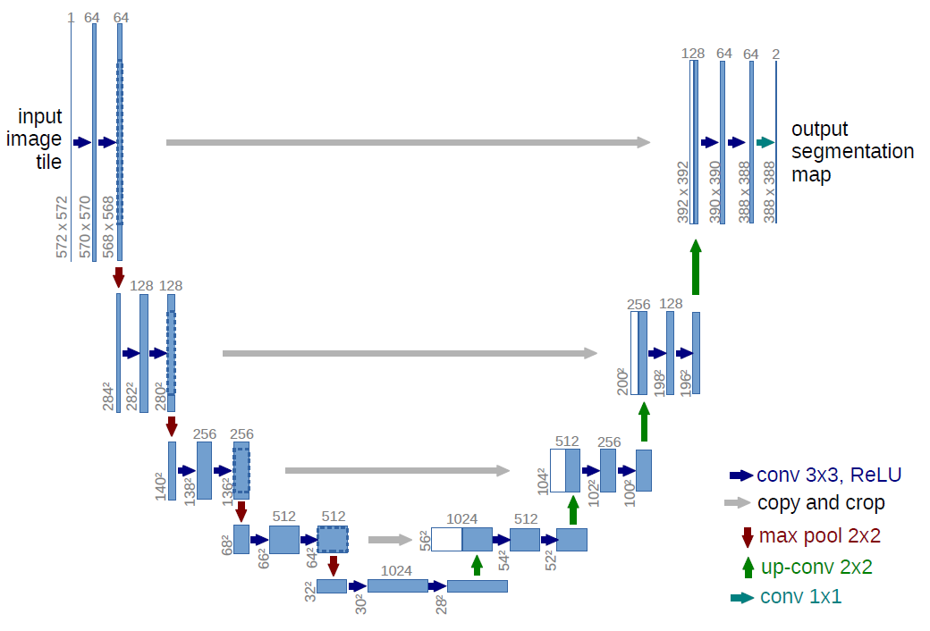
The U-Net model architecture was first introduced in the 2015 paper U-Net: Convolutional Networks for Biomedical Image Segmentation by Olaf Ronneberger, Philipp Fischer and Thomas Brox. The name U-Net comes from the shape of the model in the schematic that the original authors drew. See above. It is debatable if this is the best choice of name. There are other ways to represent the model and this name obscures the main features. A U-Net model can best be described as a convolutional autoencoder with skip connections (also called residual connections). Here is a linear representation that shows this more clearly, where the skip connections form the U’s:
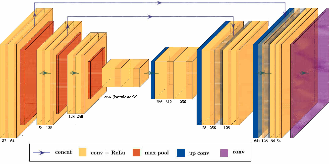
None the less, the name U-Net has come to mean exactly this in literature - a convolutional autoencoder with skip connections. Therefore I’ll keep using the name.1
Many papers and websites still cite the original 2015 paper. However this model should be seen as a “grandfather” to more recent versions. It is hard to tell from papers what their actual models look like. Looking at the reference code we find several improvements on the original design (e.g. no cropping) and many different kinds of layers which differ from codebase to codebase. Furthermore there is usually flexibility with various parameters of the model.
I’ve seen a U-Net model described as “stacking layers like Lego bricks”. It is really up to you to decide what is best and what layers you want to use. It is an open question what value any of the more complex layers provide. At the very least what can be said is that in machine learning brute force wins over targeted optimisation: for more complex tasks bigger and deeper models are preferable.
But to summarise, we can say that a U-Net model has three primary features:
- It is primarily made up of convolutional layers.
- It has layers which downsample the image height and width while increasing the channels followed by layers which upsample the height and width while decreasing the channels.
- It has skip connections between the “down” side and “up” side.
The second point is what makes it an autoencoder. It is worth reading theories on the latent space of variational autoencoders which justifies the whole model architecture.
Architecture
This is the model architecture that will be implemented here. It is based on PyTorch models by OpenAI and LucidRains.
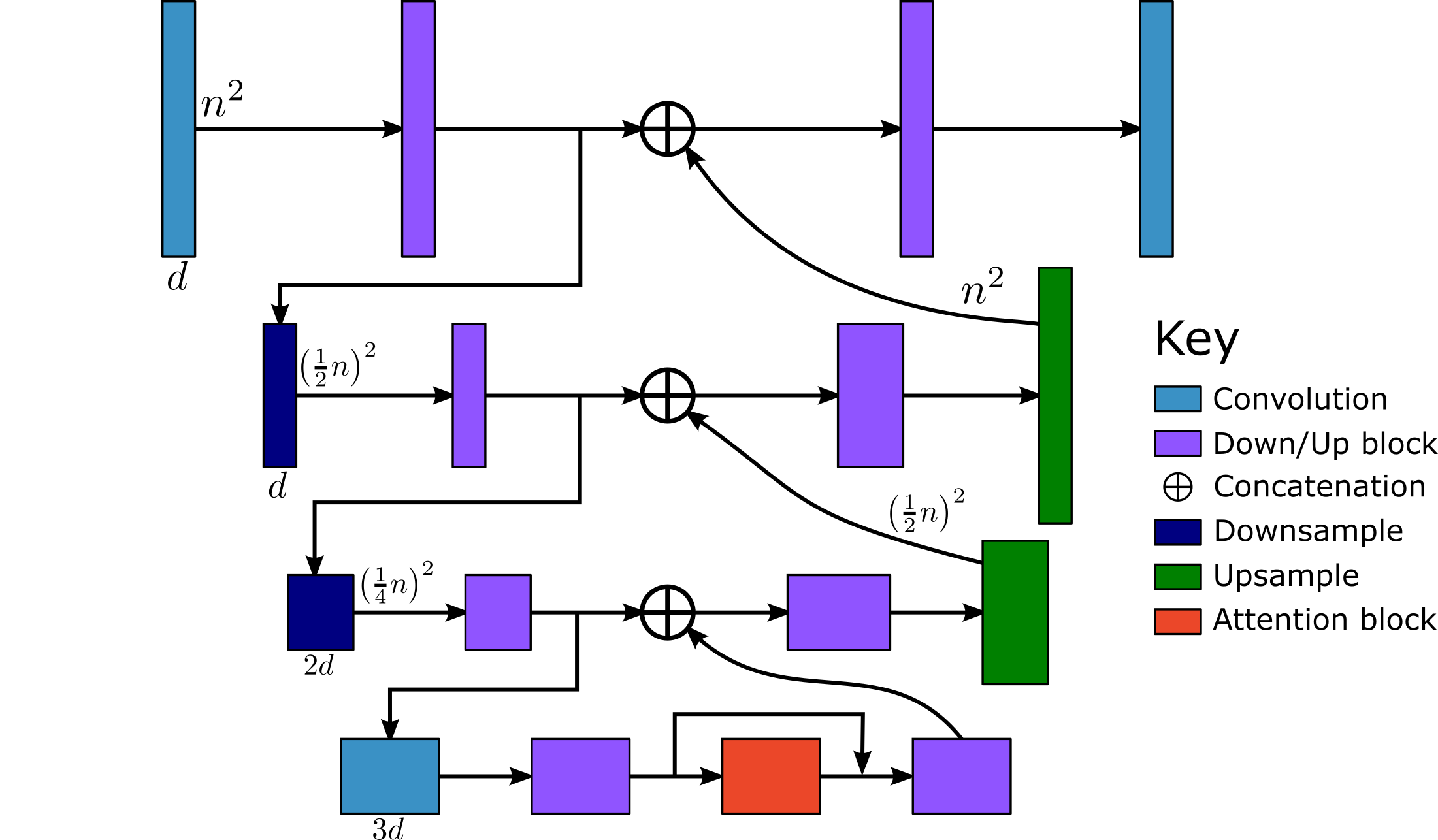
Each downsample layer will decrease the image height and width by a factor of 2 but increase the channel dimension by a multiplication factor $m$. The sample is therefore downscaled by an overall factor of $\tfrac{1}{2}\tfrac{1}{2}(m)=\tfrac{m}{4}$ per level. This is reversed with the upsample layers. The model however is based on convolutional layers whose size are independent of the input image height and width and only depend on the channel dimension. (The inference time is a factor of the image size.) Each layer grows with a factor $d^2$ for a channel dimension $d$. Therefore the largest layers are the middle (bottom) layers where the channel dimension is largest. Also because of the concatenation on the channel dimension, the upside layers will tend to be much larger than their downside counterparts.
This figure shows this exponential relationship with the channel dimension:
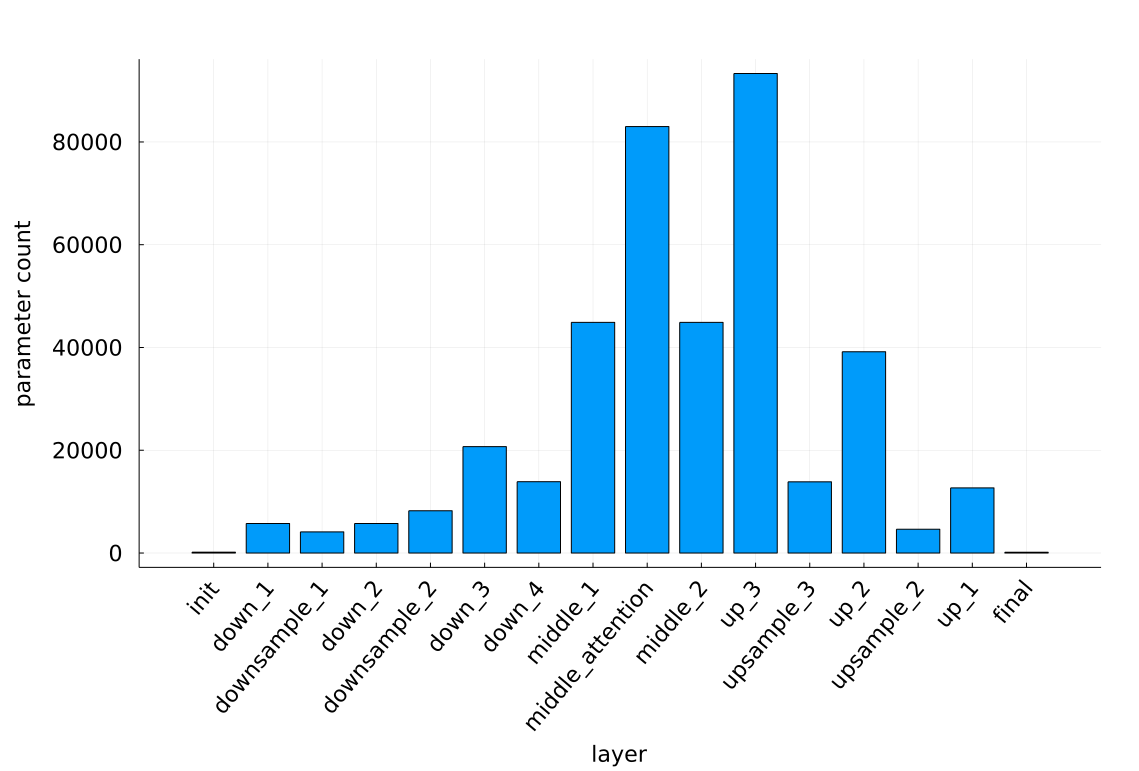
So despite the symmetrical nature of the schematic, the model is not very symmetric.
The rest of this section will detail the code for the model in a top-down fashion. For the full model see UNet.jl. Please see this source code for the printing functions, which are not detailed here.
The blocks used in the model are described in the next section, Blocks.
A slight problem
There is a slight problem with making the U-Net model in Julia. The reference models are based in PyTorch and the code unfortunately cannot be directly translated because of restrictions in the Julia language. The PyTorch implementations use an array for the skip connections. They append to it on the down side and then pop values out on the up side. The Julia machine libary Flux however does not support these mutating array operations in backward passes.
Here is a minimum working example.
Define the model and a basic forward pass:
struct UNet{D<:Tuple,U<:Tuple}
    downs::D
    ups::U
end

function (u::UNet)(x::AbstractArray)
    h = AbstractArray[]
    for block in u.downs
        x = block(x)
        push!(h, x)
    end
    for block in u.ups
        x = cat(x, pop!(h), dims=3)
        x = block(x)
    end
    x
end
Test the forward pass using a very basic model:
using Flux
X = randn(Float32, 10, 10, 1, 1)
model = UNet(
    (Conv((3, 3), 1 => 1, stride=(1, 1), pad=(1, 1)),),
    (Conv((3, 3), 2 => 1, stride=(1, 1), pad=(1, 1)),),
)
y = model(X)
This works. However during training we need to apply the backward pass. Here is an example of that:
y, pull = Flux.pullback(model, X)
errors = randn(size(y)...)
grads = pull(errors)
The last line will result in this error:
ERROR: Mutating arrays is not supported -- called pop!(Vector{AbstractArray}, ...)
This error occurs when you ask Zygote to differentiate operations that change
the elements of arrays in place (e.g. setting values with x .= ...)

Possible fixes:
- avoid mutating operations (preferred)
- or read the documentation and solutions for this error
  https://fluxml.ai/Zygote.jl/latest/limitations
There are three solutions:
- Avoid using the mutating operation all together.
- Write a custom ChainRulesCore.rrule for the operation.
- Manually write the backward pass instead of using automatic differentiation.
Option 2 is best when the operation can be isolated to only one layer.2 However here it encompasses most of the forward pass so it essentially is the same as option 3. Option 3 is not a good idea because (1) it requires much more work and (2) the forward pass and backward pass will not be automatically in sync.
So we are left with option 1. There are two ways to implement it. The first is to fix the amount of layers so that we don’t need a mutable array. For example, for the minimum working example with only two layers:
function (u::UNet)(x::AbstractArray)
    h = u.downs[1](x)
    h = cat(h, h, dims=3)
    h = u.ups[1](h)
    h
end
The backward pass code will now work.
For a full working example, see my UNetFixed model at UNetFixed.jl.
The second is to embrace that Julia is a functional programming language and use a functional approach.
We can use a Flux.SkipConnection layer to implement the skip connection.
This will lead to a much more flexible model and hence is the construction that will be described in the remainder of this post.
For example:
model = Chain(
    Conv((3, 3), 1 => 1, stride=(1, 1), pad=(1, 1)),
    SkipConnection(
        identity,  # *rest of model here*
        (x, y) -> cat(x, y, dims=3)
    ),
    Conv((3, 3), 2 => 1, stride=(1, 1), pad=(1, 1)),
)
Again the backward pass code will now work.
For a model with multiple skip connections we can nest layers recursively.
Conditional SkipConnection
As in part 1 we need to pass two inputs to the model and so we’ll need to reuse the ConditionalChain from
part 1.
We’ll need a custom ConditionalSkipConnection layer which can handle multiple inputs too.
The source code for Flux.SkipConnection can easily be adapted for this:
struct ConditionalSkipConnection{T,F} <: AbstractParallel
    layers::T
    connection::F
end

Flux.@functor ConditionalSkipConnection

function (skip::ConditionalSkipConnection)(x, ys...)
    skip.connection(skip.layers(x, ys...), x)
end
Constructor
The model is all held in a struct:
struct UNet{E,C<:ConditionalChain}
    time_embedding::E
    chain::C
    num_levels::Int
end

Flux.@functor UNet (time_embedding, chain,)
The model will have a complex constructor. The most important parameters are the number of in channels (1 for a grey image and 3 for RGB images), the model dimension $d$ and the number of time steps $T$. The total number of parameters scales with $d^2$. So if we double the model channel we will quadruple the number of parameters.
Additionally, the user will also be able to specify the channel multipliers instead of the default value of 2 per level.
The block layer (purple blocks) will be configurable (either a ConvEmbed or a ResBlock) as well as the number of (purple) blocks per level.
As a simplification only the last block in each level will be connected to a skip connection.
We will have Flux.GroupNorm layers which requires a number of groups G; this will be set the same throughout the model.
Lastly we’ll have a parameter for the attention layer.
function UNet(
    in_channels::Int,
    model_channels::Int,
    num_timesteps::Int
    ;
    channel_multipliers::NTuple{N,Int}=(1, 2, 4),
    block_layer=ResBlock,
    num_blocks_per_level::Int=1,
    block_groups::Int=8,
    num_attention_heads::Int=4
) where {N}
    model_channels % block_groups == 0 ||
        error("The number of block_groups ($(block_groups)) must divide the number of model_channels ($model_channels)")

    channels = [model_channels, map(m -> model_channels * m, channel_multipliers)...]
    in_out = collect(zip(channels[1:end-1], channels[2:end]))
There are many different variations of the time embedding layer.
This is one used by LuicidRains.
For the SinusoidalPositionEmbedding see part 1-sinusodial embedding.
    time_dim = 4 * model_channels
    time_embed = Chain(
        SinusoidalPositionEmbedding(num_timesteps, time_dim),
        Dense(time_dim, time_dim, gelu),
        Dense(time_dim, time_dim)
    )
Next we’ll make the up and down blocks, where we can have more than one per level. The keys will be very useful when we print the entire model:
    in_ch, out_ch = in_out[1]
    down_keys = num_blocks_per_level == 1 ? [Symbol("down_1")] : [Symbol("down_1_$(i)") for i in 1:num_blocks_per_level]
    up_keys = num_blocks_per_level == 1 ? [Symbol("up_1")] : [Symbol("up_1_$(i)") for i in 1:num_blocks_per_level]
    down_blocks = [
        block_layer(in_ch => in_ch, time_dim; groups=block_groups) for i in 1:num_blocks_per_level
    ]
    up_blocks = [
        block_layer((in_ch + out_ch) => out_ch, time_dim; groups=block_groups),
        [block_layer(out_ch => out_ch, time_dim; groups=block_groups) for i in 2:num_blocks_per_level]...
    ]
Here is the chain constructor.
We have an initial convolution to transform the image so that it has $d$ channels.
The final convolution reverses this.
In between are the down blocks, the skip connection and the up blocks.
The skip connection calls the recursive function _add_unet_level (to be defined shortly).
    chain = ConditionalChain(;
        init=Conv((3, 3), in_channels => model_channels, stride=(1, 1), pad=(1, 1)),
        NamedTuple(zip(down_keys, down_blocks))...,
        down_1=block_layer(in_ch => in_ch, time_dim; groups=block_groups),
        skip_1=ConditionalSkipConnection(
            _add_unet_level(in_out, time_dim, 2;
                block_layer=block_layer,
                block_groups=block_groups,
                num_attention_heads=num_attention_heads,
                num_blocks_per_level=num_blocks_per_level
            ),
            cat_on_channel_dim
        ),
        NamedTuple(zip(up_keys, up_blocks))...,
        final=Conv((3, 3), model_channels => in_channels, stride=(1, 1), pad=(1, 1))
    )
Recursion should not be overused for making a model. We’ll only go four levels deep.
Finally, build the struct:
    UNet(time_embed, chain, length(channel_multipliers) + 1)
end
Here is the cat_on_channel_dim function:
cat_on_channel_dim(h::AbstractArray, x::AbstractArray) = cat(x, h, dims=3)And here is the _add_unet_level function.
As always for recursive functions, start with the break condition for the recursion else enter in a recursive loop:
function _add_unet_level(in_out::Vector{Tuple{Int,Int}}, emb_dim::Int, level::Int;
    block_layer, num_blocks_per_level::Int, block_groups::Int, num_attention_heads::Int
)
    if level > length(in_out) # stop recursion and make the middle
        in_ch, out_ch = in_out[end]
        keys_ = (Symbol("down_$level"), :middle_1, :middle_attention, :middle_2)
        layers = (
            Conv((3, 3), in_ch => out_ch, stride=(1, 1), pad=(1, 1)),
            block_layer(out_ch => out_ch, emb_dim; groups=block_groups),
            SkipConnection(MultiheadAttention(out_ch, nhead=num_attention_heads), +),
            block_layer(out_ch => out_ch, emb_dim; groups=block_groups),
        )
    else # recurse down a layer
        in_ch_prev, out_ch_prev = in_out[level-1]
        in_ch, out_ch = in_out[level]
        down_keys = num_blocks_per_level == 1 ? [Symbol("down_$(level)")] : [Symbol("down_$(level)_$(i)") for i in 1:num_blocks_per_level]
        up_keys = num_blocks_per_level == 1 ? [Symbol("up_$(level)")] : [Symbol("up_$(level)_$(i)") for i in 1:num_blocks_per_level]
        keys_ = (
            Symbol("downsample_$(level-1)"),
            down_keys...,
            Symbol("skip_$level"),
            up_keys...,
            Symbol("upsample_$level")
        )
        down_blocks = [
            block_layer(in_ch => in_ch, emb_dim; groups=block_groups) for i in 1:num_blocks_per_level
        ]
        up_blocks = [
            block_layer((in_ch + out_ch) => out_ch, emb_dim; groups=block_groups),
            [block_layer(out_ch => out_ch, emb_dim; groups=block_groups) for i in 2:num_blocks_per_level]...
        ]
        layers = (
            downsample_layer(in_ch_prev => out_ch_prev),
            down_blocks...,
            ConditionalSkipConnection(
                _add_unet_level(in_out, emb_dim, level + 1;
                    block_layer=block_layer,
                    block_groups=block_groups,
                    num_attention_heads=num_attention_heads,
                    num_blocks_per_level=num_blocks_per_level
                ),
                cat_on_channel_dim
            ),
            up_blocks...,
            upsample_layer(out_ch => in_ch),
        )
    end
    ConditionalChain((; zip(keys_, layers)...))
end
Forward pass
For the forward pass we calculate the time embedding and pass it along with the input to the chain.
function (u::UNet)(x::AbstractArray, timesteps::AbstractVector{Int})
    emb = u.time_embedding(timesteps)
    h = u.chain(x, emb)
    h
end
Full model
in_channels = 1
model_channels = 16
num_timesteps = 100
model = UNet(in_channels, model_channels, num_timesteps;
    block_layer=ResBlock,
    num_blocks_per_level=1,
    block_groups=8,
    channel_multipliers=(1, 2, 3),
    num_attention_heads=4
)

x = randn(Float32, 28, 28, 1, 10);
t = rand(1:num_timesteps, 10);
y = model(x, t)
Printing the full model takes 181 lines. (Please see the source code for the printing functions.) See UNet.txt. Here is a condensed version:
UNet(
  time_embedding = Chain(
    SinusoidalPositionEmbedding(100 => 64),
    Dense(64 => 64, gelu),              # 4_160 parameters
    Dense(64 => 64),                    # 4_160 parameters
  ),
  chain = ConditionalChain(
    init = Conv((3, 3), 1 => 16, pad=1),  # 160 parameters
    down_1 = ResBlock(16 => 16),          # 5744 parameters
    skip_1 = ConditionalSkipConnection(
      ConditionalChain(
        downsample_1 = Conv((4, 4), 16 => 16, pad=1, stride=2),  # 4_112 parameters
        down_2 = ResBlock(16 => 16),      # 5744 parameters
        skip_2 = ConditionalSkipConnection(
          ConditionalChain(
            downsample_2 = Conv((4, 4), 16 => 32, pad=1, stride=2),  # 8_224 parameters
            down_3 = ResBlock(32 => 32),   # 20_704 parameters
            skip_3 = ConditionalSkipConnection(
              ConditionalChain(
                down_4 = Conv((3, 3), 32 => 48, pad=1),  # 13_872 parameters
                middle_1 = ResBlock(48 => 48), # 44_880 parameters
                middle_attention = SkipConnection(
                  MultiheadAttention(),       # 82_992 parameters
                  +,
                ),
                middle_2 = ResBlock(48 => 48), # 44_880 parameters
              ),
              DenoisingDiffusion.cat_on_channel_dim,
            ),
            up_3 = ResBlock(80 => 48),  # 93_312 parameters
            upsample_3 = Chain(),       # 13_856 parameters
          ),
          DenoisingDiffusion.cat_on_channel_dim,
        ),
        up_2 = ResBlock(48 => 32),     # 39_168 parameters
        ),
        upsample_2 = Chain(),  # 4_624 parameters
      ),
      DenoisingDiffusion.cat_on_channel_dim,
    ),
    up_1 = ResBlock(32 => 16),        #12_672 parameters
    final = Conv((3, 3), 16 => 1, pad=1),  # 145 parameters
  ),
)         # Total: 107 trainable arrays, 403_409 parameters,
          # plus 1 non-trainable, 6_400 parameters, summarysize 1.592 MiB.
Blocks
For the final scripts please see DenoisingDiffusion.jl/src/models. Please also see these scripts for the printing functions which are not detailed here.
Convolution
This post assumes you already have a knowledge of convolutional layers. Otherwise this post on Convolutional Neural Networks is a good source with a nice animation. This repository has nice animations on the effects of altering the stride and padding.
For an image input size $i$ (either the height or width), kernel/filter size $k$, padding $p$ and stride $s$, the output image will have size:
\[o=\left\lfloor{\frac{i + 2p - k}{s} + 1} \right\rfloor \tag{3.1} \label{eq:conv}\]Choosing $p=1$, $s=1$ and $k=3$ ensures that the output size is the same as the input size, $o=i$.
Let the input channel size be $d_i$ and the output channel size be $d_o$. The convolutional layer has $d_o$ kernels of size $k \cdot k \cdot d_i$ each with a bias of size $d_o$. Therefore the layer has $(k^2d_i + 1)d_o$ parameters. For $d_i = m_id$ and $d_o=m_od$ where $m_i$ and $m_o$ are the input and output channel multipliers respectively, the number of parameters is approximately $k^2m_im_od^2$.
ConvEmbed
The ConvEmbed block will form the main block layer.
It will perform a convolution on the input and add the time embedding.
Additionally it will apply a GroupNorm, adjust the time embedding for a layer specific embedding and apply an activation function.
The output is equivalent to activation(norm(conv(x)) .+ embed_layers(emb)).
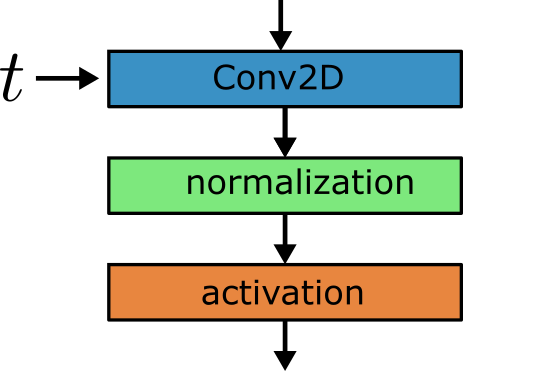
This has one convolution with $(3^2d_i + 1)d_o$ parameters, one fully connected layer with $(d_e+1)d_o$ parameters and a group norm with $2d_o$ parameters. For $d_i=m_id$, $d_o=m_od$ and $d_e=4d$, the number of parameters is approximately $(9m_i+4)m_od^2$. For the up layers $m_i$ will be a combination of two multipliers because of the concatenation: $m_i = m_t + m_{t-1}$.
This table summarises the resultant block sizes (all values are a slight underestimate):
| down | up | |||||
|---|---|---|---|---|---|---|
| level | $m_i$ | $m_o$ | size ($d^2$) | $m_i$ | $m_o$ | size ($d^2$) |
| 1 | 1 | 1 | 13 | 1+1 | 1 | 22 |
| 2 | 1 | 1 | 13 | 2+1 | 2 | 62 |
| 3 | 2 | 2 | 44 | 3+2 | 3 | 147 |
| 4 | 3 | 3 | 93 | |||
Constructor:
struct ConvEmbed{E,C<:Conv,N,A} <: AbstractParallel
    embed_layers::E
    conv::C
    norm::N
    activation::A
end

Flux.@functor ConvEmbed

function ConvEmbed(channels::Pair{<:Integer,<:Integer}, emb_channels::Int; groups::Int=8, activation=swish)
    out = channels[2]
    embed_layers = Chain(
        swish,
        Dense(emb_channels, out),
    )
    conv = Conv((3, 3), channels, stride=(1, 1), pad=(1, 1))
    norm = GroupNorm(out, groups)
    ConvEmbed(embed_layers, conv, norm, activation)
end
Forward pass. The embedding is reshaped so that each embedding value is applied to the whole cross-section at each channel for each batch:
function (m::ConvEmbed)(x::AbstractArray, emb::AbstractArray)
    h = m.conv(x)
    h = m.norm(h)
    emb_out = m.embed_layers(emb)
    num_ones = length(size(h)) - length(size(emb_out))
    emb_out = reshape(emb_out, (repeat([1], num_ones)..., size(emb_out)...))
    h = h .+ emb_out
    h = m.activation(h)
    h
end
We can now use this ConvEmbed block as our block layer in the U-Net Constructor.
ResBlock
Instead of a single ConvEmbed block we can use a more complex Resnet style block which connects two blocks with a skip connection.
Only the first block will have the time embedding.
A complication of this block is that the input channels can be different to the output channels, so an extra convolution is needed to make the skip connection the same size.
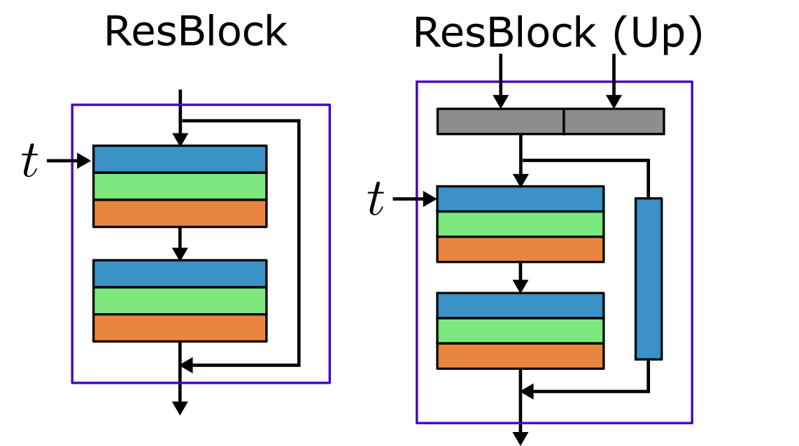
The ConvEmbed block has approximately $(9m_i+4)m_od^2$ parameters, the convolution layer has approximately $3^2m_o^2d^2$ and
the skip connection has approximately $3^2m_im_od^2$ where $m_i\neq m_o$.
In total there are $(9(m_i+m_o) + 4)m_od^2$ parameters on the down blocks and $(9(2m_i+m_o) + 4)m_od^2$ on the up blocks.
This table summarises the resultant block sizes (all values are a slight underestimate):
| down | up | |||||
|---|---|---|---|---|---|---|
| level | $m_i$ | $m_o$ | size ($d^2$) | $m_i$ | $m_o$ | size ($d^2$) |
| 1 | 1 | 1 | 22 | 1+1 | 1 | 49 |
| 2 | 1 | 1 | 22 | 2+1 | 2 | 152 |
| 3 | 2 | 2 | 80 | 3+2 | 3 | 363 |
| 4 | 3 | 3 | 174 | |||
The constructor:
struct ResBlock{I<:ConvEmbed,O,S} <: AbstractParallel
    in_layers::I
    out_layers::O
    skip_transform::S
end

Flux.@functor ResBlock

function ResBlock(channels::Pair{<:Integer,<:Integer}, emb_channels::Int; groups::Int=8, activation=swish)
    out_ch = channels[2]
    conv_timestep = ConvEmbed(channels, emb_channels; groups=groups, activation=activation)
    out_layers = Chain(
        Conv((3, 3), out_ch => out_ch, stride=(1, 1), pad=(1, 1)),
        GroupNorm(out_ch, groups),
        activation,
    )
    if channels[1] == channels[2]
        skip_transform = identity
    else
        skip_transform = Conv((3, 3), channels, stride=(1, 1), pad=(1, 1))
    end
    ResBlock(conv_timestep, out_layers, skip_transform)
end
Forward pass:
function (m::ResBlock)(x::AbstractArray, emb::AbstractArray)
    h = m.in_layers(x, emb)
    h = m.out_layers(h)
    h = h + m.skip_transform(x)
    h
end
Down sampling
The original U-Net used a 2×2 MaxPool layer for the down sampling. This samples the maximum value from every 2×2 window so that the output is $o=\left \lfloor \frac{i}{2} \right \rfloor$. Using Flux it is made with:
MaxPool((2, 2))By default the stride is also 2×2. There are no parameters.
By looking at equation $\ref{eq:conv}$, we can also make a down sample layer by setting $k=4$, $s=2$ and $p=1$. The result is then also $o=\left \lfloor \frac{i}{2} \right \rfloor$. This is the method I’ve chosen to use:
function downsample_layer(channels::Pair{<:Integer,<:Integer})
    Conv((4, 4), channels, stride=(2, 2), pad=(1, 1))
end
This is a convolution layer with $16m_im_od^2+m_od$ parameters.
If the input image has an odd length then the downsample dimension will be $\frac{i-1}{2}$. Then if we upsample back by 2 the size will be $i-2$ instead of $i$ and the concatenation will fail. So the image has to be evenly divisible by powers of 2 in the forward pass.
Up sampling
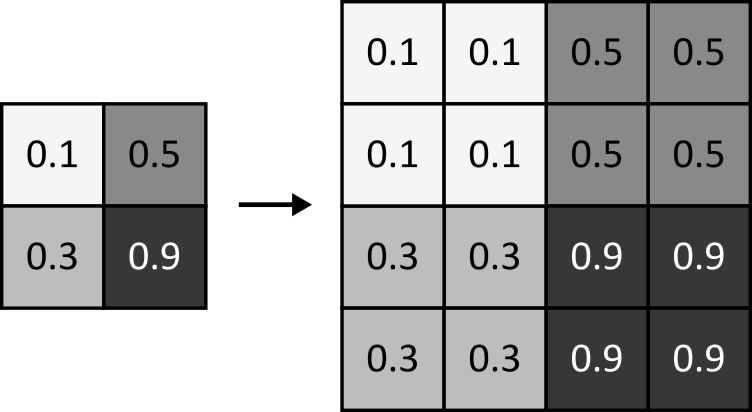
Here the strategy is to first apply nearest neighbour upsampling followed by a convolution. In nearest neighbour upsampling we take each value and copy them to 2×2 cells. Hence the image will increase from an initial input dimension $i$ to an output dimension $o=2i$.
function upsample_layer(channels::Pair{<:Integer,<:Integer})
    Chain(
        Upsample(:nearest; scale=(2, 2)),
        Conv((3, 3), channels, stride=(1, 1), pad=(1, 1))
    )
end
There are $9m_om_id^2+m_od$ parameters from the convolution.
Another technique uses a transpose convolution layer. This can be made with ConvTranspose((2,2), 1=>1, stride=(2,2)).
This however is not recommended because of the “checkerboard” effect that transpose convolutions suffer from.
Attention
This is the most complicated block in the model and also the largest. This block is based on the transformer self-attention layer that was first introduced in Google’s 2017 paper Attention is all you need. Ho et. al. do not give a justification for including it in the model.
For a full discussion of self-attention please see my earlier post on transformers.
Unfortunately we can’t reuse all the code exactly. The biggest difference is that the attention is applied across channels (groups of 2D images) whereas for transformers they are applied across the embedding dimension (words). So here we take in a $W \times H \times C \times B$ input and rearrange it into $d_h \times WH \times h \times B$ arrays. For language models we take in a $d \times N \times B$ input and rearrange it into $d_h \times N \times h \times B$ arrays.
This version uses convolutions instead of dense layers for the query, key and value matrices and the output matrix. The query, key and value are all combined into one convolution with $3^2(md)(3md)=27m^2d^2$ parameters (no bias). The output has $9m^2d^2+md$ parameters. So in total this layer has approximately $36m^2d^2$ parameters.
Define the struct:
struct MultiheadAttention{Q<:Conv,O<:Conv}
    nhead::Int
    to_qkv::Q
    to_out::O
end

Flux.@functor MultiheadAttention (to_qkv, to_out,)
Constructor:
function MultiheadAttention(dim_model::Int, dim_head::Int; nhead::Int=4)
    dim_hidden = dim_head * nhead
    MultiheadAttention(
        nhead,
        Conv((3, 3), dim_model => dim_hidden * 3, stride=(1, 1), pad=(1, 1), bias=false),
        Conv((3, 3), dim_hidden => dim_model, stride=(1, 1), pad=(1, 1))
    )
end

function MultiheadAttention(dim_model::Int; nhead::Int=4)
    if dim_model % nhead != 0
        error("model dimension=$dim_model is not divisible by number of heads=$nhead")
    end
    MultiheadAttention(dim_model, div(dim_model, nhead), nhead=nhead)
end
Forward pass:
function (mha::MultiheadAttention)(x::A) where {T,A<:AbstractArray{T,4}}
    # batch multiplication version. Input is W × H × C × B
    qkv = mha.to_qkv(x)
    Q, K, V = Flux.chunk(qkv, 3, dims=3)

    c = size(Q, 3)
    dh = div(c, mha.nhead)
    #size(Q) == (W, H, dh*nhead, B) => (W*H, dh, nhead, B) => (dh, W*H, nhead, B)
    Q = permutedims(reshape(Q, :, dh, mha.nhead, size(x, 4)), [2, 1, 3, 4])
    K = permutedims(reshape(K, :, dh, mha.nhead, size(x, 4)), [2, 1, 3, 4])
    V = permutedims(reshape(V, :, dh, mha.nhead, size(x, 4)), [2, 1, 3, 4])
    #size(attn) == (dh, W*H, nhead, B)
    attn = scaled_dot_attention(Q, K, V)
    #size(attn) == (dh, W*H, nhead, B) => (W*H, dh, nhead, B) => (W, H, dh*nhead, B)
    attn = permutedims(attn, [2, 1, 3, 4])
    attn = reshape(attn, size(x, 1), size(x, 2), c, size(x, 4))

    mha.to_out(attn)
end

function (mha::MultiheadAttention)(x::A) where {T,A<:AbstractArray{T,3}}
    # single sample. Make it a batch of 1
    x = reshape(x, size(x)..., 1)
    attn = mha(x)
    reshape(attn, size(attn)[1:end-1]...)
end
Scaled dot attention (same as for the transformer):
function scaled_dot_attention(query::A1, key::A2, value::A3) where {
    T,A1<:AbstractArray{T,4},A2<:AbstractArray{T,4},A3<:AbstractArray{T,4}}
    # Batched version. Input is (dh, N, nhead, B)
    dh = size(query, 1)
    scale = one(T) / convert(T, sqrt(dh))
    keyT = permutedims(key, (2, 1, 3, 4)) # important: don't use a view (PermutedDimsArray) because this slows batched_mul
    sim = scale .* batched_mul(keyT, query) #size(sim) == (N, N, nhead, B)
    sim = softmax(sim; dims=1)
    batched_mul(value, sim) #size(attention) == (dh, N, nhead, B)
end
Batched multiplication (same as for the transformer):
function batched_mul(A::AbstractArray{T,4}, B::AbstractArray{T,4}) where {T}
    if (size(A, 2) != size(B, 1)) || (size(A, 3) != size(B, 3)) || (size(A, 4) != size(B, 4))
        message = "A has dimensions $(size(A)) but B has dimensions $(size(B))"
        throw(DimensionMismatch(message))
    end
    new_A = reshape(A, size(A, 1), size(A, 2), :)
    new_B = reshape(B, size(B, 1), size(B, 2), :)
    C = batched_mul(new_A, new_B)
    new_C = reshape(C, (size(C, 1), size(C, 2), size(A, 3), size(A, 4)))
    new_C
end
Accounting
The following is a summary of all the (approximate) equations for the parameters:
| Type | Parameters |
|---|---|
| Conv | $k^2 m_i m_o d^2 +m_o d$ |
| ConvEmbed | $(9 m_i + 4)m_o d^2$ |
| ResBlock | $(9(m_i + m_o) + 4)m_o d^2 $ |
| ResBlock (up) | $(9(2m_i + m_o) + 4)m_o d^2 $ |
| Downsample | $16m_i m_od^2 +m_o d$ |
| Upsample | $9m_i m_od^2 +m_o d$ |
| Attention | $36m_i^2d^2 + m_i d$ |
With these we can construct a table for the full UNet model:
| Key | Type | $m_i$ | $m_o$ | $d^2$ | |
|---|---|---|---|---|---|
| 1 | init | Conv | 0 | 1 | 0 |
| 2 | down_1 | ResBlock | 1 | 1 | 22 |
| 3 | downsample_1 | Conv | 1 | 1 | 16 |
| 4 | down_2 | ResBlock | 1 | 1 | 22 |
| 5 | downsample_2 | Conv | 1 | 2 | 32 |
| 6 | down_3 | ResBlock | 2 | 2 | 80 |
| 7 | down_4 | Conv | 2 | 3 | 54 |
| 8 | middle_1 | ResBlock | 3 | 3 | 174 |
| 9 | middle_attention | MultiHeadAttention | 3 | 3 | 324 |
| 10 | middle_2 | ResBlock | 3 | 3 | 174 |
| 11 | up_3 | ResBlock | 5 | 3 | 363 |
| 12 | upsample_3 | Conv | 3 | 2 | 54 |
| 13 | up_2 | ResBlock | 3 | 2 | 152 |
| 14 | upsample_2 | Conv | 2 | 1 | 18 |
| 15 | up_1 | ResBlock | 2 | 1 | 49 |
| 16 | final | Conv | 1 | 0 | 0 |
| Total | 1 | 1 | 1534 |
Setting model_channels to $d=16$ results in $1534d^2=392,704$ parameters which is 97.3% of the true total of 403,409.
The difference comes from ignoring bias terms and terms in $d$.
MNIST
Load data
We can load data using the MLDatasets.jl package.
The first call to MNIST will download the data (approximately 11 MB) to data_directory.
using MLDatasets

data_directory = "path/to/MNIST"
trainset = MNIST(Float32, :train, dir=data_directory)
testset = MNIST(Float32, :test, dir=data_directory)
Some quick data exploration:3
nrows = 3
canvases = []
for label in 0:9
    idxs = (1:length(trainset))[trainset.targets .== label]
    for idx in rand(idxs, nrows)
        img = convert2image(trainset, trainset.features[:, :, idx])
        push!(canvases, plot(img))
    end
end
canvases = [canvases[nrows * j + i] for i in 1:nrows for j in 0:9]
plot(canvases..., layout=(nrows, 10), ticks=nothing)
Normalise the dataset (function defined in part 1):
norm_data = normalize_neg_one_to_one(reshape(trainset.features, 28, 28, 1, :))Forward diffusion
We can mostly reuse the code from part 1.
The one difference is that we’ll be using a cosine schedule for the $\beta_t$’s instead of a linear schedule. This was proposed in the 2021 paper Improved Denoising Diffusion Probabilistic Models by Alex Nichol snd Prafulla Dhariwal. The authors found that this schedule more evenly distributes noise over the whole time range for images.
The formula for $\bar{\alpha}_t$ is:
\[\bar{\alpha}_t = \frac{f(t)}{f(0)}, \quad f(t) = \cos\left(\frac{t/T+s}{1+s}\frac{\pi}{2}\right)^2\]They set $s=0.008$. Each $\alpha_t$ can then be calculated as \(\frac{\bar{\alpha}_{t}}{\bar{\alpha}_{t-1}}\) and hence $ \beta_t = 1 - \alpha_t $.
In code:
function cosine_beta_schedule(num_timesteps::Int, s=0.008)
    t = range(0, num_timesteps; length=num_timesteps + 1)
    α_cumprods = (cos.((t / num_timesteps .+ s) / (1 + s) * π / 2)) .^ 2
    α_cumprods = α_cumprods / α_cumprods[1]
    βs = 1 .- α_cumprods[2:end] ./ α_cumprods[1:(end-1)]
    clamp!(βs, 0, 0.999)
    βs
end
Forward diffusion:
num_timesteps = 100
βs = cosine_beta_schedule(num_timesteps, 0.008)
diffusion = GaussianDiffusion(Vector{Float32}, βs, (28, 28, 1,), identity)

X = norm_data[:, :, :, idx]
canvases = []
for frac in [0.0, 0.25, 0.5, 0.75, 1]
    local p
    timestep = max(1, ceil(Int, frac * num_timesteps))
    Xt = q_sample(diffusion, X, timestep)
    clamp!(Xt, -one(Xt[1]), one(Xt[1]))
    img = convert2image(trainset, normalize_zero_to_one(Xt[:, :, 1, 1]))
    p = plot(img, title="t=$timestep")
    push!(canvases, p)
end

p = plot(canvases..., layout=(1, 5), link=:both, size=(900, 200))
The result:

Training
For the full training script, see train_images.jl. I also have made a Jupyter Notebook hosted on Google Colab available at DenoisingDiffusion-MNIST.ipynb.4
Firstly split the training dataset into train and validation sets. The test dataset will be used for the evaluating the model after training is finished.
function split_validation(rng::AbstractRNG, data::AbstractArray; frac=0.1)
    nsamples = size(data)[end]
    idxs = randperm(rng, nsamples)
    ntrain = nsamples - floor(Int, frac * nsamples)
    data[:, :, :, idxs[1:ntrain]], data[:, :, :, idxs[(ntrain+1):end]]
end

train_x, val_x = split_validation(MersenneTwister(seed), norm_data)
Create the model:
in_channels = size(train_x, 3)
data_shape = size(train_x)[1:3]
model_channels = 16
num_timesteps = 100
model = UNet(in_channels, model_channels, num_timesteps;
    block_layer=ResBlock,
    num_blocks_per_level=1,
    block_groups=8,
    channel_multipliers=(1, 2, 3),
    num_attention_heads=4
)
βs = cosine_beta_schedule(num_timesteps, 0.008)
diffusion = GaussianDiffusion(Vector{Float32}, βs, data_shape, model)
Train the model using the functions from part 1-training:
train_data = Flux.DataLoader(train_x |> to_device; batchsize=32, shuffle=true);
val_data = Flux.DataLoader(val_x |> to_device; batchsize=32, shuffle=false);
loss(diffusion, x) = p_losses(diffusion, loss_type, x; to_device=to_device)
opt = Adam(learning_rate)
output_directory = "outputs\\MNIST_" * Dates.format(now(), "yyyymmdd_HHMM")
opt_state = Flux.setup(opt, diffusion)
history = train!(
    loss, diffusion, train_data, opt_state, val_data
    ; num_epochs=20
)
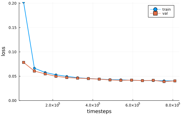
The training history:
Reverse diffusion
Sample:
Xs, X0s = p_sample_loop_all(diffusion, 16; to_device=cpu);Here is the resulting reverse process (left) and first image estimates made using the U-Net model (right):5
Evaluation
We would now like to evaluate how good our image generation model is. In part 1 we had a clear defined target - a spiral defined by mathematical equations - and hence a clear defined measure of error: the shortest distance from each point to the spiral. Here our sample should be recognisable as one of 10 digits without ambiguity. At the same time it should not match any in the original dataset because we want to create new images. This makes it tricky to evaluate.
Here I propose two techniques. The first is the mean Euclidean distance compared to the mean test images. The second is the Fréchet LeNet Distance, inspired by the popular Fréchet Inception Distance (FID). Both require generating a large amount of samples for statistical significance. I have generated 10,000 samples to match the 10,000 test data samples.
For a notebook with the full code please see MNIST-test.ipynb.
MNIST means
We can calculate the mean test images using:
mnist_means = []
for label in 0:9
    idxs = testset.targets .== label
    x_mean = mean(testset.features[:, :, idxs], dims=3)
    push!(mnist_means, x_mean[:, :, 1])
endAs an aside, the generated sample means tend to be remarkably close to these test set means. This may be because the U-Net model is only used for $\tilde{\mu}_t$ and not $\tilde{\beta}_t$ in the reverse equations.
Define the distance as the minimum of the mean Euclidean distance of $x$ to each mean $\bar{x}_k$:
\[d = \min_{0 \leq k \leq 9} \frac{1}{WH}\sqrt{\sum_{i}^W\sum_{j}^H (x_{ij} - \bar{x}_{k,ij})^2}\]The score is then the average of $d$ over all samples.
In code:
function average_min_distances(X, x_means)
    num_samples = size(X, 4)
    n_means = length(mean_imgs)
    distances = fill(Inf, num_samples)
    labels = fill(-1, num_samples)
    for i in 1:num_samples
        x = X[:, :, 1, i]
        for k in 0:9
            distance_k = sqrt(sum(abs2, x - x_means[k + 1])) / length(x)
            if (distance_k < distances[i])
                labels[i] = k
                distances[i] = distance_k
            end
        end
    end
    mean(distances), [count(x->x==label, labels) for label in 0:9]
end
Sample values look like:
| dataset | score |
|---|---|
| test | 0.0080 |
| train | 0.0080 |
| generated | 0.0084 |
| random | 0.0913 |
The counts per label look like:
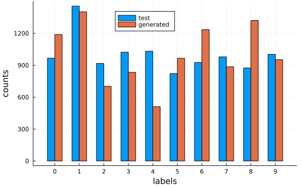
The test set labels are only 82% accurate, so this method is not good enough for a bias free evaluation.
Frechet LeNet Distance
A smarter way to evaluate the model is the Fréchet Inception Distance (FID). This was introduced in the 2017 paper GANs Trained by a Two Time-Scale Update Rule Converge to a Local Nash Equilibrium by Heusel et. al.. There are two important insights. Firstly, image classification can be considered a solved task after the work of the last two decades in machine learning. That is we can use an image classification model to get insights into our generated data. Secondly, we can view the outputs of penultimate layer of the model as a probability distribution and compare the statistical distance of it between different datasets. The intuition behind using the penultimate layer is that it is an abstract feature space containing essential information about the samples that we can for comparison rather than manually specifying features.
In particular, the FID score uses the Inception V3 model as the classification model and the Fréchet Distance as the statistical measure:
\[d(\mathcal{N}(\mu_1, \Sigma_1^2), \mathcal{N}(\mu_2, \Sigma_2^2)) = ||\mu_1 - \mu_2||^2 + \text{trace}\left(\Sigma_1 + \Sigma_2 -2\left( \Sigma_1 \Sigma_2 \right)^{1/2} \right) \label{eq:Frechet} \tag{4.7}\]Intuitively the first term represents the distance between the means and the second term counts for a difference in variances.
The Inception V3 model however is overkill here. It has over 27 million parameters and the penultimate layer has a length of 2048. My proposal is to instead use the smaller LeNet-5 with 44,000 parameters and an output length of 84. It was first proposed in the 1998 paper Gradient-Based Learning Applied to Document Recognition by Yann LeCun, Leon Bottou, Yoshua Bengio and Patrick Haffner.
This is a Julia implementation from the Flux model zoo:
function LeNet5()
    out_conv_size = (28÷4 - 3, 28÷4 - 3, 16)
    return Chain(
            Conv((5, 5), 1=>6, relu),
            MaxPool((2, 2)),
            Conv((5, 5), 6=>16, relu),
            MaxPool((2, 2)),
            Flux.flatten,
            Dense(prod(out_conv_size), 120, relu),
            Dense(120, 84, relu),
            Dense(84, 10)
          )
end
Training this model should be covered in any introductory machine Learning material. You can view my attempt at train_classifier.jl. This model gets a test accuracy of 98.54%. This is good enough for us to consider it a perfect oracle.
After training we can load the model:
classifier_path = "models\\LeNet5\\model.bson"
classifier = BSON.load(classifier_path)[:model]
To use the generated outputs we’ll have to normalise them between 0 and 1 (function defined in part 1-spiral dataset):
for i in 1:n_samples
    global X_generated
    X_generated[:, :, :, i] = normalize_zero_to_one(X_generated[:, :, :, i])
end
We can apply our classifier to the normalised generated outputs and compare label counts to the test data:
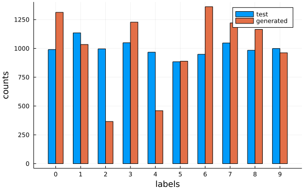
We can immediately see that our model has a bias to producing 0s and 6s and produces too few 2s and 4s.
Now for the FLD score. We can implement equation $\ref{eq:Frechet}$ in Julia as follows:6
function gaussian_frechet_distance(μ1::AbstractMatrix, Σ1::AbstractMatrix, μ2::AbstractMatrix, Σ2::AbstractMatrix)
    diff = μ1 - μ2
    covmean = sqrt(Σ1 * Σ2)
    if eltype(covmean) <: Complex
        @warn("sqrt(Σ1 * Σ2) is complex")
        if all(isapprox.(0.0, diag(imag(covmean)), atol=1e-3))
            @info("imaginary components are small and have been set to zero")
            covmean = real(covmean)
        end
    end
    sum(diff .* diff) + tr(Σ1 + Σ2 - 2 * covmean)
end
Usage:
classifier_headless = classifier[1:(end - 1)]
activations = classifier_headless(X_generated)
activations_test = classifier_headless(X_test)
μ = mean(activations; dims=2)
Σ = cov(activations; dims=2, corrected=true)
μ_test = mean(activations_test; dims=2)
Σ_test = cov(activations_test; dims=2, corrected=true)
fld = gaussian_frechet_distance(μ_test, Σ_test, μ, Σ)
Sample values:
| dataset | score |
|---|---|
| test | 0.0001 |
| train | 0.4706 |
| generated | 23.8847 |
| random | 337.7282 |
Our generated dataset is indeed significantly better than random. However it is still noticeably different from the original dataset.
Conclusion
The main focus of this post was to build a U-Net model. It is general purpose and can be used for other image generation tasks. For example, I did try to generate Pokemon with it, inspired by This Pokémon Does Not Exist but unfortunately did not get good results. You can see my notebooks at github.com/LiorSinai/DenoisingDiffusion-examples.
Now that we can generate numbers the next task is to tell the model which number we want. That way we can avoid the bias towards certain numbers that was evidenced in the evaluation. This will be the focus of the third and final part on Classifier-free guidance. That same method is used with text embeddings to direct the outcome of AI art generators.
Now that our models are getting large, it is also desirable to improve the generation time. This can be accomplished with a technique introduced in the paper Denoising Diffusion Implicit Models (DDIM) by Jiaming Song, Chenlin Meng and Stefano Ermon. DDIM sampling allows the model to skip timesteps during image generation. This results in much faster image generation with a trade off of a minor loss in quality. I have implemented DDIM sampling in my code. Please review this if you are interested.
-
One has to admit it has the added advantage of being very short. ↩
-
For an example of this, see the “backpropagation for mul4d” card in an earlier post on transformers. ↩
-
The
convert2imagecode can be rewritten as:function img_WH_to_gray(img_WH::AbstractArray{T,N}) where {T,N} @assert N == 2 || N == 3 img_HW = permutedims(img_WH, (2, 1, 3:N...)) img = Images.colorview(Images.Gray, img_HW) img end -
Google Colab does not natively support Julia so you’ll have to install it every time you run the notebook. Plots.jl does not work on Google Colab. ↩
-
I’ve used a function to combine multiples images into one:
function combine(imgs::AbstractArray, nrows::Int, ncols::Int, border::Int) canvas = zeros(Gray, 28 * nrows + (nrows+1) * border, 28 * ncols + (ncols+1) * border) for i in 1:nrows for j in 1:ncols left = 28 * (i-1) + 1 + border * i right = 28 * i + border * i top = 28 * (j - 1) + 1 + border * j bottom = 28 * j + border * j canvas[left:right, top:bottom] = imgs[:, :, ncols * (i-1) + j] end end canvas end -
The one tricky part of the equation is the matrix square root $A^{1/2}$, defined as a matrix $B=A^{1/2}$ such that $BB=A$. In code it is therefore important to realise that
sqrt.(A)andsqrt(A)are very different operations. ↩
