Classifier-free guidance for denoising diffusion probabilistic model in Julia.
Update 28 August 2023: code refactoring and update to Flux 0.13.11 explicit syntax.
This is part of a series. The other articles are:
Full code available at github.com/LiorSinai/DenoisingDiffusion.jl. Examples notebooks at github.com/LiorSinai/DenoisingDiffusion-examples. Google Colab training notebook at DenoisingDiffusion-MNIST.ipynb.
Table of Contents
Introduction
A major disadvantage of the models developed so far is that the output is random. The user has no way to control it. For the pattern in part 1, we always have to create a spiral. For the number generation in part 2, we cannot specify which number we want. However it is easy enough to extend the existing code to include guidance where the user can specify the output. This post details the conditioning and classifier-free guidance techniques to accomplish this. It applies them to the 2D pattern generation and number generation problems from the previous posts.
These same techniques are very powerful when combined with other models. For example, we can use a model to generate text embeddings and pass these to the diffusion model, creating a text-to-image workflow. This is the underlying idea behind all the popular AI art generators like Stable Diffusion, DALLE-2 and Imagen.
Guided diffusion
Conditioning
We already have time embeddings and we can combine other sorts of embeddings with it. These embeddings can be added, multiplied or concatenated to the time embeddings. So instead of estimating the noise $\epsilon_\theta(x_t | t)$ we’ll estimate $\epsilon_\theta(x_t | t, y)$ where $y$ is the label of the class. We can also directly pass in the conditioning parameters (text embeddings) $c$ and estimate $\epsilon_\theta(x_t | t, c)$.
It is still useful for this guided model to generate random samples. This gives it backwards compatibility with our previous code and as we’ll see shortly, gives us a reference point for increasing the conditioning signal. We can do this by passing a special label/embedding denoting the empty set $\emptyset$. Mathematically we can write $\epsilon_\theta(x_t | t) = \epsilon_\theta(x_t | t, \emptyset)$. During training we sometimes randomly change the label/embedding to the empty set label/embedding so that model learns to associate it with random choice.
In practice when conditioning on the label, the first column of the embedding matrix (label 0 in Python or label 1 in Julia) is reserved for the empty set and the rest are used for the classes. Or when conditioning on the embedding vectors directly, a vector of all zeros can be used for the empty set.
Classifier-free guidance
Conditioning on its own works well enough for the toy problems in this blog series. However for text-to-image models we need a stronger signal, and so need a way of amplifying this conditioning. This is known as guidance.
An early proposal for guided diffusion was classifier guidance in the paper Diffusion Models Beat GANs on Image Synthesis by Prafulla Dhariwal and Alex Nichol. This technique used a classifier model to estimate a gradient through a loss function which was then added to the estimate of the sample:
\[\mu_t = \tilde{\mu}_t(x_t | y) + s\Sigma_\theta(x_t | y)\nabla_{x_t} \log p_\phi (y | x_t) \tag{2.1}\]Where $ \mu_t $ is the mean sample per time step, $y$ is the target class, $s$ is the guidance scale, $\Sigma_\theta$ is the model variance and $\nabla_{x_t} \log p_\phi$ is the gradient of the log-probability of the output of the classifier.1 This is an incredibly complicated solution. Creating a classifier model is easy (see part 2-Frechet LeNet Distance) but creating a classifier model that can work throughout all the noisy time steps of diffusion is very difficult. This requires a second U-Net model that needs to be trained in parallel.
Thankfully a much simpler and more effective solution was proposed in the 2022 paper Classifier-Free Diffusion Guidance by Jonathan Ho and Tim Salimans. They proposed estimating the noise twice per time step: once with conditioning parameters (text embeddings) and once without. The predicted noise $\epsilon_\theta$ is then given as a weighted sum of the two:
\[\begin{align} \epsilon_\theta(x_t, c) &= (1 + s)\epsilon_\theta(x_t | c) - s\epsilon_\theta(x_t) \\ &= \epsilon_\theta(x_t | c) + s(\epsilon_\theta(x_t | c) - \epsilon_\theta(x_t)) \tag{2.2} \end{align}\]Where $t$ is the time step, $x_t$ is the sample, $c$ are the conditioning parameters and $s$ is the guidance scale. From the second line we can see that the gradient is estimated as the difference between the noise with conditioning $\epsilon_\theta(x_t | c)$ and the noise without conditioning $\epsilon_\theta(x_t)$. It is then added to the original noise term, essentially telling it very crudely “go in this direction”. This is an incredibly simple idea but it is effective.
Nichol et. al. quickly adapted this technique, realising it was superior to their complicated classifier guidance. They made the minor improvement of putting the unconditioned noise $\epsilon_\theta(x_t)$ as the first term:
\[\epsilon_\theta(x_t, c) = \epsilon_\theta(x_t) + s(\epsilon_\theta(x_t | c) - \epsilon_\theta(x_t)) \tag{2.3} \label{eq:classifier-free-guidance}\]This form makes slightly more intuitive sense, as we are taking the random noise and guiding it with the gradient, rather than guiding the conditioned (and already guided) noise with the gradient. Then for the special case of $s=1$, $\epsilon_\theta(x_t, c) = \epsilon_\theta(x_t | c)$. That is just plain conditioning. This is significant because it means that for $s=1$ we can use conditioning without estimating the noise twice for classifier-free guidance.
We can now implement this in Julia. We can reuse the same functions and use multiple dispatch to differentiate between them: the guided versions will have three inputs ($x_t$, $t$, $c$) while the originals will have two ($x_t$, $t$).
For the full code see guidance.jl.
Reverse diffusion
This is the guided version of the reverse process from part 1.
For text embeddings coming from a language model the new argument to p_sample would be a matrix.
However here the embeddings are calculated in the model too, so p_sample will expect a vector of integer labels instead.
These will then be passed to an embedding layer.
(For modifications which can take in external embeddings, see the feature/external-embeddings branch on the repository.)
A label of 1 will be considered random choice and other integers will correspond to the classes.
As discussed above, for the special case of the guidance_scale=1 inputs will be passed directly to the model.
Otherwise the more computationally intensive classifier-free guidance will be invoked.
function p_sample(
    diffusion::GaussianDiffusion, x::AbstractArray, timesteps::AbstractVector{Int}, labels::AbstractVector{Int}, noise::AbstractArray;
    clip_denoised::Bool=true, add_noise::Bool=true, guidance_scale::AbstractFloat=1.0f0
    )
    if guidance_scale == 1.0f0
        x_start, pred_noise = denoise(diffusion, x, timesteps, labels)
    else
        x_start, pred_noise = classifier_free_guidance(
            diffusion, x, timesteps, labels; guidance_scale=guidance_scale
        )
    end
    if clip_denoised
        clamp!(x_start, -1, 1)
    end
    posterior_mean, posterior_variance = q_posterior_mean_variance(diffusion, x_start, x, timesteps)
    x_prev = posterior_mean
    if add_noise
        x_prev += sqrt.(posterior_variance) .* noise
    end
    x_prev, x_start
end
We need a new method for the denoise function to handle three inputs:
function denoise(
    diffusion::GaussianDiffusion,
    x::AbstractArray, timesteps::AbstractVector{Int}, labels::AbstractVector{Int}
    )
    noise = diffusion.denoise_fn(x, timesteps, labels)
    x_start = predict_start_from_noise(diffusion, x, timesteps, noise)
    x_start, noise
end
Next is the implementation of classifier-free guidance with equation $\ref{eq:classifier-free-guidance}$. This code calculates the conditioned noise and the unconditioned noise at the same time.
function classifier_free_guidance(
    diffusion::GaussianDiffusion,
    x::AbstractArray, timesteps::AbstractVector{Int}, labels::AbstractVector{Int}
    ; guidance_scale=1.0f0
)
    T = eltype(eltype(diffusion))
    guidance_scale_ = convert(T, guidance_scale)
    batch_size = size(x)[end]
    x_double = cat(x, x, dims=ndims(x))
    timesteps_double = vcat(timesteps, timesteps)
    labels_both = vcat(labels, fill(1, batch_size))

    noise_both = diffusion.denoise_fn(x_double, timesteps_double, labels_both)
    inds = ntuple(Returns(:), ndims(x_double) - 1)
    ϵ_cond = view(noise_both, inds..., 1:batch_size)
    ϵ_uncond = view(noise_both, inds..., (batch_size+1):(2*batch_size))
    noise = ϵ_uncond + guidance_scale_ * (ϵ_cond - ϵ_uncond)

    x_start = predict_start_from_noise(diffusion, x, timesteps, noise)
    x_start, noise
end
All the other functions remain the same as in part 1.
Full loop
This is the guided version of the sampling loops from part 1.
Sampling loops with an extra input:
function p_sample_loop(
    diffusion::GaussianDiffusion, shape::NTuple, labels::AbstractVector{Int}
    ; clip_denoised::Bool=true, to_device=cpu, guidance_scale::AbstractFloat=1.0f0
)
    T = eltype(eltype(diffusion))
    x = randn(T, shape) |> to_device
    @showprogress "Sampling ..." for i in diffusion.num_timesteps:-1:1
        timesteps = fill(i, shape[end]) |> to_device
        noise = randn(T, size(x)) |> to_device
        x, x_start = p_sample(
            diffusion, x, timesteps, labels, noise
            ; clip_denoised=clip_denoised, add_noise=(i != 1), guidance_scale=guidance_scale
        )
    end
    x
end

function p_sample_loop(diffusion::GaussianDiffusion, batch_size::Int, label::Int; options...)
    labels = fill(label, batch_size)
    p_sample_loop(diffusion, (diffusion.data_shape..., batch_size), labels; options...)
end

function p_sample_loop(diffusion::GaussianDiffusion, labels::AbstractVector{Int}; options...)
    batch_size = length(labels)
    p_sample_loop(diffusion, (diffusion.data_shape..., batch_size), labels; options...)
end
Sampling loop returning all diffusion time steps and $x_0$ estimates:
function p_sample_loop_all(
    diffusion::GaussianDiffusion, shape::NTuple, labels::AbstractVector{Int}
    ; clip_denoised::Bool=true, to_device=cpu, guidance_scale::AbstractFloat=1.0f0
)
    T = eltype(eltype(diffusion))
    x = randn(T, shape) |> to_device
    x_all = Array{T}(undef, size(x)..., 0) |> to_device
    x_start_all = Array{T}(undef, size(x)..., 0) |> to_device
    dim_time = ndims(x_all)
    @showprogress "Sampling..." for i in diffusion.num_timesteps:-1:1
        timesteps = fill(i, shape[end]) |> to_device
        noise = randn(T, size(x)) |> to_device
        x, x_start = p_sample(
            diffusion, x, timesteps, labels, noise
            ; clip_denoised=clip_denoised, add_noise=(i != 1), guidance_scale=guidance_scale
        )
        x_all = cat(x_all, x, dims=dim_time)
        x_start_all = cat(x_start_all, x_start, dims=dim_time)
    end
    x_all, x_start_all
end

function p_sample_loop_all(diffusion::GaussianDiffusion, batch_size::Int, label::Int; options...)
    labels = fill(label, batch_size)
    p_sample_loop_all(diffusion, (diffusion.data_shape..., batch_size), labels; options...)
end

function p_sample_loop_all(diffusion::GaussianDiffusion, labels::AbstractVector{Int}; options...)
    batch_size = length(labels)
    p_sample_loop_all(diffusion, (diffusion.data_shape..., batch_size), labels; options...)
end
Training
This is the guided version of the training process from part 1.
As before we’ll have two methods for p_losses.
The first takes in the four inputs (x_start, timesteps, noise and the new labels) and calculates the losses:
function p_losses(
    diffusion::GaussianDiffusion, loss, x_start::AbstractArray{T,N},
    timesteps::AbstractVector{Int}, labels::AbstractVector{Int}, noise::AbstractArray
) where {T,N}
    if (size(x_start, N) != length(labels))
        throw(DimensionMismatch("batch size != label length, $N != $(length(labels))"))
    end
    x = q_sample(diffusion, x_start, timesteps, noise)
    model_out = diffusion.denoise_fn(x, timesteps, labels)
    loss(model_out, noise)
end
The second will generate the timesteps and noise based on x_start (as before):
function p_losses(
    diffusion::GaussianDiffusion,
    loss,
    x_start::AbstractArray,
    labels::AbstractVector{Int},
    ; to_device=cpu
    )
    batch_size = size(x_start)[end]
    @assert(batch_size == length(labels),
        "batch size != label length, $batch_size != $(length(labels))"
    )
    timesteps = rand(1:diffusion.num_timesteps, batch_size) |> to_device
    noise = randn(eltype(eltype(diffusion)), size(x_start)) |> to_device
    p_losses(diffusion, loss, x_start, timesteps, labels, noise)
end
The training loop needs to be updated so that it can randomly set labels to that of the empty set $\emptyset$.2
This train! function from part 1 is extended as follows:
using Flux: DataLoader
using ProgressMeter

function train!(loss, model, data::DataLoader, opt_state;
    num_epochs::Int=10,
    prob_uncond::Float64=0.0,
    )
    history = Dict("mean_batch_loss" => Float64[],)
    for epoch = 1:num_epochs
        progress = Progress(length(data); desc="epoch $epoch/$num_epochs")
        total_loss = 0.0
        for (idx, x) in enumerate(data)
            if (x isa Tuple)
                y = prob_uncond == 0.0 ?
                    x[2] :
                    randomly_set_unconditioned(x[2]; prob_uncond=prob_uncond)
                x_splat = (x[1], y)
            else
                x_splat = (x,)
            end
            batch_loss, grads = Flux.withgradient(model) do m
                loss(m, x_splat...)
            end
            total_loss += batch_loss
            Flux.update!(opt_state, model, grads[1])
            ProgressMeter.next!(progress)
        end
        push!(history["mean_batch_loss"], total_loss / length(data))
        @printf("mean batch loss: %.5f ; ", history["mean_batch_loss"][end])
    end
    history
end

function randomly_set_unconditioned(
    labels::AbstractVector{Int}; prob_uncond::Float64=0.20
    )
    # with probability prob_uncond we train without class conditioning
    labels = copy(labels)
    batch_size = length(labels)
    is_not_class_cond = rand(batch_size) .<= prob_uncond
    labels[is_not_class_cond] .= 1
    labels
end
For more functionality like calculating the validation loss after each epoch, see the train.jl script in the repository.
That’s it. Our code can now do guided diffusion. Let’s test it out on both the 2D patterns and the number generation.
2D patterns
Generate data
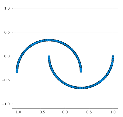
In part 1 we only worked with a spiral dataset. However we can work other patterns too. Here is a Julia implementation of the Scikit-learn moon dataset:
function make_moons(rng::AbstractRNG, n_samples::Int=1000)
    n_moons = floor(Int, n_samples / 2)
    t_min = 0.0
    t_max = π
    t_inner = rand(rng, n_moons) * (t_max - t_min) .+ t_min
    t_outer = rand(rng, n_moons) * (t_max - t_min) .+ t_min
    outer_circ_x = cos.(t_outer)
    outer_circ_y = sin.(t_outer)
    inner_circ_x = 1 .- cos.(t_inner)
    inner_circ_y = 1 .- sin.(t_inner) .- 0.5

    data = [outer_circ_x outer_circ_y; inner_circ_x inner_circ_y]
    permutedims(data, (2, 1))
end

make_moons(n_samples::Int=1000) = make_moons(Random.GLOBAL_RNG, n_samples)
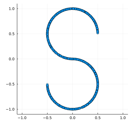
Similarly for the Scikit-learn s-curve:
function make_s_curve(rng::AbstractRNG, n_samples::Int=1000)
    t = 3 * π * (rand(rng, n_samples) .- 0.5)
    x = sin.(t)
    y = sign.(t) .* (cos.(t) .- 1)
    permutedims([x y], (2, 1))
end

make_s_curve(n_samples::Int=1000) = make_s_curve(Random.default_rng(), n_samples)
Then we can make and combine samples of all three:
n_batch = 9_000
num_classes = 3
nsamples_per_class = round(Int, n_batch / num_classes)
X1 = normalize_neg_one_to_one(make_spiral(nsamples_per_class));
X2 = normalize_neg_one_to_one(make_s_curve(nsamples_per_class));
X3 = normalize_neg_one_to_one(make_moons(nsamples_per_class));
X = hcat(X1, X2, X3)
Plotting all at once:

Make the labels. Remember that 1 is reserved for random choice.
labels = 1 .+ vcat(
    fill(1, nsamples_per_class),
    fill(2, nsamples_per_class),
    fill(3, nsamples_per_class),
    )
Model
We can use the same model as part 1-sinusodial embeddings with an additional Flux.Embedding layer at each level.
Otherwise no other changes required.
model = ConditionalChain(
    Parallel(
        .+, Dense(2, d_hid),
        Chain(
            SinusoidalPositionEmbedding(num_timesteps, d_hid),
            Dense(d_hid, d_hid)
        ),
        Embedding(1 + num_classes => d_hid)
    ),
    swish,
    Parallel(
        .+,
        Dense(d_hid, d_hid),
        Chain(
            SinusoidalPositionEmbedding(num_timesteps, d_hid),
            Dense(d_hid, d_hid)
        ),
        Embedding(1 + num_classes => d_hid)
    ),
    swish,
    Parallel(
        .+,
        Dense(d_hid, d_hid),
        Chain(
            SinusoidalPositionEmbedding(num_timesteps, d_hid),
            Dense(d_hid, d_hid)
        ),
        Embedding(1 + num_classes => d_hid)
    ),
    swish,
    Dense(d_hid, 2),
)
Results patterns
Training is the same as part 1-training. The only difference is that the loss function must now take in three arguments:
loss(diffusion, x, y) = p_losses(diffusion, loss_type, x, y; to_device=to_device)See train_generated_2d_cond.jl for the full script.
We can sample at a guidance scale of 1 to avoid classifier-free guidance:
num_samples = 1000
x_gen = Dict{Int, Dict{Symbol, Array{Float32, 3}}}()
γ = 1.0f0
for label in 1:4
    Xs, X0s = p_sample_loop_all(diffusion, 1000, label; guidance_scale=γ, clip_denoised=false)
    x_gen[label] = Dict(
        :Xs => Xs,
        :X0s => X0s
    )
end
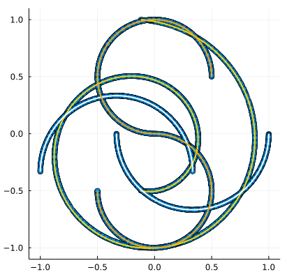
The result:
The random choice label of 1 will result in a combination of all the patterns. This is because the 2D points are sampled from one of the patterns independently of their neighbours. It is therefore highly unlikely that they will all be randomly chosen from one pattern.
MNIST
Load data
The MNIST dataset comes with labels. We will have to shift them over by 2 because 1 is reserved for random choice and so 0 needs to correspond to 2.
The code:
trainset = MNIST(Float32, :train, dir=data_directory);
norm_data = normalize_neg_one_to_one(reshape(trainset.features, 28, 28, 1, :));
labels = 2 .+ trainset.targets; # 1->default, 2->0, 3->1, ..., 9->11
We need a new method for split_validation to split the labels too:
function split_validation(rng::AbstractRNG, data::AbstractArray, labels::AbstractVector{Int}; frac=0.1)
    nsamples = size(data)[end]
    idxs = randperm(rng, nsamples)
    ntrain = nsamples - floor(Int, frac * nsamples)
    train_data = (data[:, :, :, idxs[1:ntrain]], labels[idxs[1:ntrain]])
    val_data = (data[:, :, :, idxs[(ntrain+1):end]], labels[idxs[(ntrain+1):end]])
    train_data, val_data
end
train_x, val_x = split_validation(MersenneTwister(seed), norm_data, labels);
UNetConditioned
We would like to use the same model from part 2-constructor.
However we need to add two extra elements to the struct: a new embedding layer and a function to combine embeddings.
The combine_embeddings can be one of + (as used above for the spiral), * or vcat.
It should not have parameters.
The new struct is:
struct UNetConditioned{E1,E2,F,C<:ConditionalChain}
    time_embedding::E1
    class_embedding::E2
    combine_embeddings::F
    chain::C
    num_levels::Int
end

Flux.@functor UNetConditioned (time_embedding, class_embedding, chain,)
The constructor is almost the same, so I’ll skip most of it:
function UNetConditioned(
    in_channels::Int,
    model_channels::Int,
    num_timesteps::Int,
    ;
    num_classes::Int=1,
    channel_multipliers::NTuple{N,Int}=(1, 2, 4),
    block_layer=ResBlock,
    num_blocks_per_level::Int=1,
    block_groups::Int=8,
    num_attention_heads::Int=4,
    combine_embeddings=vcat
) where {N}
    ...

    class_embedding = Flux.Embedding((num_classes + 1) => time_dim)
    embed_dim = (combine_embeddings == vcat) ? 2 * time_dim : time_dim
    # use embed_dim instead of time_dim

    ...
    UNetConditioned(time_embed, class_embedding, combine_embeddings, chain, length(channel_multipliers) + 1)
end
The forward pass has additional steps for calculating the class embedding and combining it with the time embeddings:
function (u::UNetConditioned)(x::AbstractArray, timesteps::AbstractVector{Int}, labels::AbstractVector{Int})
    time_emb = u.time_embedding(timesteps)
    class_emb = u.class_embedding(labels)
    emb = u.combine_embeddings(time_emb, class_emb)
    h = u.chain(x, emb)
    h
end
Automatically set labels to random choice if none are supplied:
function (u::UNetConditioned)(x::AbstractArray, timesteps::AbstractVector{Int})
    batch_size = length(timesteps)
    labels = fill(1, batch_size)
    u(x, timesteps, labels)
end
For printing functions please see UNetConditioned.jl.
We can make a model with:
in_channels = 1
model_channels = 16
num_timesteps = 100
num_classes = 10 #0-9
model = UNetConditioned(in_channels, model_channels, num_timesteps;
    num_classes=num_classes,
    block_layer=ResBlock,
    num_blocks_per_level=1,
    block_groups=8,
    channel_multipliers=(1, 2, 3),
    num_attention_heads=4,
    combine_embeddings=vcat
)
The whole model will have 420,497 parameters. This is only an increase of 4.3% on the unconditioned UNet.
Results MNIST
Training is the same as part 2-training. For the full training script, see train_images_cond.jl. I also have made a Jupyter Notebook hosted on Google Colab available at DenoisingDiffusion-MNIST.ipynb.3
We can now finally make the video I showed at the very top of part 1:
Xs, X0s = p_sample_loop_all(diffusion, collect(2:11); guidance_scale=2.0f0);The video:
Another interesting question to ask is what is the effect of the guidance scale on the output? Here is an image showing that:

It seems that lower guidance scale values don’t affect the output much but higher values interfere too much.
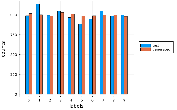
We can also go through the same exercise of calculating the Frechet LeNet Distance (FLD) from part 2-Fretchet LeNet Distance. Except this time we can ask the model to generated 1000 samples of each label. This gives us very uniform label counts:

The classifier agrees very well with our desired labels. When the guidance scale is 1 the average recall, precision and F1 score across all labels is 89%. When it is 2 the averages increase to 99%.
The FLD score is also lower. It dropped from values in the 20s without conditioning to between 4 and 8 with conditioning.
Conclusion
This three part series sought to explain the magic behind AI art generators. In particular it focused on denoising diffusion probabilistic models, the main image generation model used in text-to-image pipelines. I hope you understand them much better now and are able to experiment with your own models.
There is still ongoing controversy over AI art generators - the way training data is collected, the quality of the outputs, the potential for forgeries and debates about the value of machine generated art. As an engineer I am always tempted to promote the technology but the adverse effects of it cannot be ignored. I hope that society is able to navigate the complex questions posed by these art generators to the benefit of all involved.
One thing that is for sure is that the technology is here to stay. If you’ve followed this series properly, you’ll have a model running on your own machine training on your own data. That is not something can be taken away easily.
-
For an implementation of the classifier guidance equation, see OpenAI’s classifier_sample.py from the guided-diffusion repository. To be honest, I don’t understand this equation or the code. Why is there is a $\log$ in the gradient? Why are they computing the sum of the probabilities? ↩
-
The original code put the
randomly_set_unconditionedlogic in thep_lossesfunction. Other than that this was not the best logical place for it to be, it created the problem that this code fell under theFlux.withgradientscope and so it needed to be differentiated. HoweverZygotecan not differentiate mutating operations like.=. So instead of using:is_not_class_cond = rand(batch_size) .< prob_uncond labels[is_not_class_cond] .= 1I used:
is_class_cond = rand(batch_size) .>= prob_uncond
is_not_class_cond = .~is_class_cond
labels = (labels .* is_class_cond) + is_not_class_cond
This hack worked. However it is better to not do unnecessary differentiation. ↩
-
Google Colab does not natively support Julia so you’ll have to install it every time you run the notebook. Plots.jl does not work on Google Colab. ↩