How to calculate the statistical distance between two 2D distributions of points. But first a lesson in bad statistics, the pitfalls of visual solutions and over-complicating a solved problem.
Table of Contents
Introduction
stat. distance:0.00
A while back I was given an intriguing task: rank scatter plots by similarity. It is an unusual request but not unheard of - see this question or this one. The above is a demo of the problem at hand. (Source code.) Furthermore, there are standard statistical techniques for this sort of problem. I was drawn to the Wasserstein metric which is used in the popular Fréchet Inception Distance (FID) in machine learning. This is the “statistical distance” in the widget.
Unfortunately for me, the client came with a solution in mind already. They wanted to enclose the points in shapes and then calculate the overlap of those shapes. In more technical terms, they wanted to find convex hulls of the points and then calculate the areas of intersection between them.
I pushed back based on three points:
- The statistical properties of the polygon method are not adequate. For example, it does not handle outliers well.
- It would take too much development time and this was only one of many tasks.
-
The convex hull method would be much slower than the Wasserstein metric.
I’ve crossed out the third point because the convex hull method can be made fast. I didn’t realise this at the time. However the other two points remain valid. Thankfully the client was open to my suggestions and we did implement the Wasserstein metric. It worked well enough. (Users weren’t shown the scores; just similar plots.)
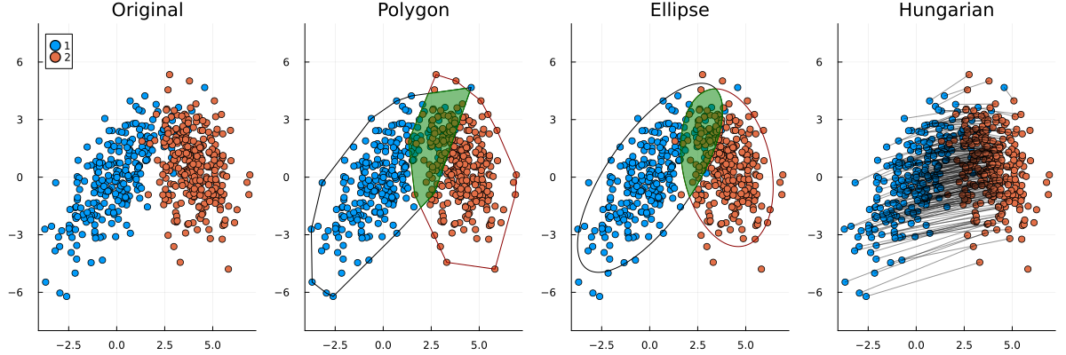
Later in my own capacity I challenged myself to try the other methods. How much more difficult was it to do the polygon method? We also brainstormed using circles and ellipses. Were these any better? This post is the outcome of that investigation.
There are too many algorithms to go into proper detail for each one. Instead I provide a high level overview and references are given for further information.
| Method | Time Complexity | Source / test LOC | Repository |
|---|---|---|---|
| Polygon | $O(nh_1 + mh_2)$ | 410 / 640 |
github.com/LiorSinai/PolygonAlgorithms.jl |
| Ellipse | $O(n+m)$ | 490 / 350 |
github.com/LiorSinai/Similarities2D |
| Hungarian | $O(n^4), n \leq m$ | 410 / 370 |
github.com/Gnimuc/Hungarian.jl, github.com/LiorSinai/AssignmentProblem.jl |
| Wasserstein | $O(n+m)$ | 30 / 0 |
github.com/LiorSinai/Similarities2D |
My implementations were done in Julia. The above table shows where the code can be viewed, the time complexity and the approximate number lines of code (LOC).1 If one bases the effort solely on LOC, the original polygon method required more than 30× the effort to the Wasserstein metric. A more detailed breakdown is available at the end in the Code analysis section.
For those who just want to compare scatter plots the right way, jump to How to compare scatter plots.
Preliminaries
Bivariate normal distributions
There are many different kinds of 2D distributions. The data that I was working with was normally distributed. This is a very common type of distribution that arises naturally in many different situation thanks to the central limit theorem. A bivariate (2D) normal distribution is described by five variables:
- The means $\mu_x$ and $\mu_y$ in the $x$ and $y$ directions respectively.
- The standard deviations $\sigma_x$ and $\sigma_y$ in the $x$ and $y$ directions respectively.
- The correlation $\rho$ between the $x$ and $y$ direction.
The widget above allows you to adjust these five variables to create many variants of this distribution.
A bivariate normal distribution with correlation $\rho$ can be constructed from two normal distributions $Z_1$ and $Z_2$ as follows:
\[X = \mu_x + \sigma_x Z_1 \\ Y = \mu_x + \sigma_y \left(\rho Z_1 + \sqrt{1-\rho^2}Z_2 \right) \label{eq:bivariate} \tag{2.1}\]Reference: www.probabilitycourse.com/chapter5/5_3_2_bivariate_normal_dist.php.
Only one of the techniques here works for any type of distribution and that is the Hungarian method, which is also the slowest. The other three assume that the underlying distributions are normally distributed.
How not to compare scatter plots
Polygons
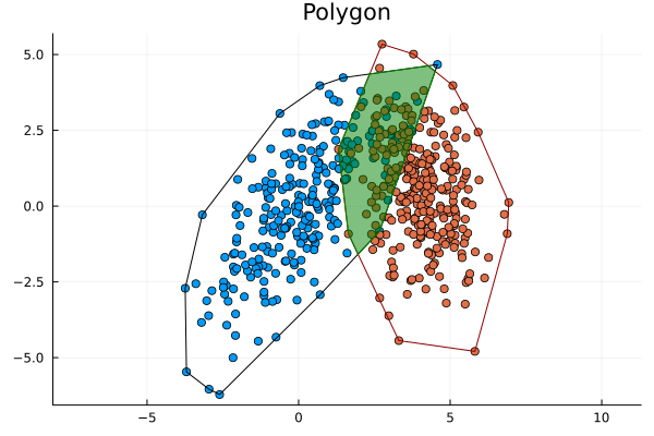
The general idea here is:
- Find convex hulls to enclose the points.
- Find the intersection of those polygons.
- Calculate the intersection over union: $\text{IoU}=\frac{A_i}{A_1 + A_2 - A_i}$.
This gives a value that varies between 0 and 1.
Finding the convex hulls is the bottleneck in this algorithm. It has a time complexity $O(nh)$ for $n$ points and $h$ points on each convex hull. Calculating the intersections once they are found is much faster: $O(h_1 + h_2)$.
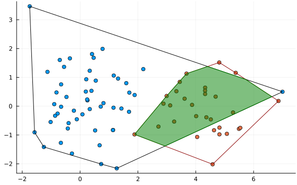
A problem with this approach is that outliers can have a dramatic effect:
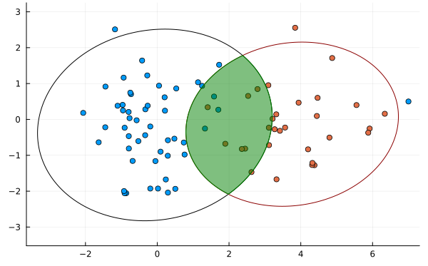
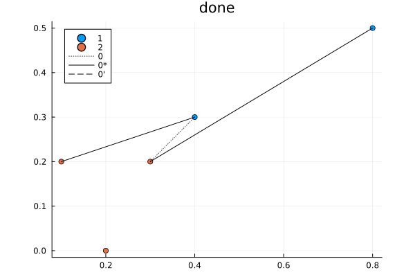
While further statistical techniques can be applied to mitigate the outlier problem, a fundamental issue is that it does not balance the contributions of means and variance well. For example, in the following image is distribution 2 or distribution 3 more similar to distribution 1?
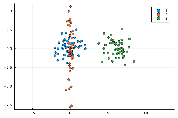
This method returns an IoU of 0 for any distribution that does not intersect it so we have no information about the third distribution.
Another difficulty with the polygon method is that polygons are described by $n$ edges. This means operations require looping through all the edges and so are of order $O(n)$ or higher, such as finding the area, the perimeter or whether or not a point lies within the polygon. Compare this to ellipses which are defined by a single equation, so all the previous operations can be found directly via formulas in $O(1)$ time.2 Another issue is that it is harder to account for all cases. Edge cases can be isolated directly in the mathematics for ellipses, but for polygons it requires actually testing each case. This is the main reason the number of tests for the polygon algorithm is much higher.
Polygons: convex hulls
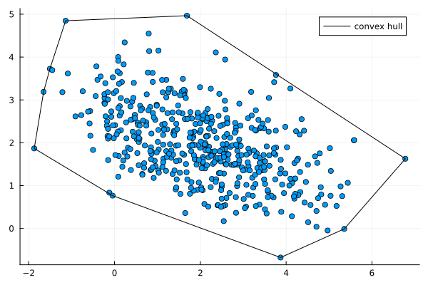
The convex hull of points in 2D is the smallest convex polygon that encloses all the points. Its edges are straight lines which connect the outermost points.
There are many algorithms to find the convex hull. The simple gift-wrapping algorithm runs in $O(nh)$ time, where $n$ is the number of points and $h$ is the number of points on the convex hull. Its worst case is $O(n^2)$ where $h=n$ - that is, all the points lie on the edge. Normally distributed points however will be the best scenario because most of the points lie inside and so $h \ll n$.
Another popular algorithm is the Graham Scan which always runs in $O(n\log n)$ time.
GeeksForGeeks have nice tutorials on both gift-wrapping and the Graham scan.
The theoretical optimal time is $O(n\log h)$. One such algorithm is Chan’s algorithm.
I choose to go with gift wrapping because it is simple and is very fast when most points lie on the inside of the convex hull.
Polygons: intersections
Finding the intersection between polygons is referred to as “polygon clipping” in computer graphics, a field where it is actually useful. There are many different polygon clipping algorithms depending on the end uses, how complex the polygons are and how many edge cases need to be catered for. A computer game which needs to process many different shapes might use the Sutherland–Hodgman algorithm whereas a vector graphics program might use the slower but more powerful Weiler-Atherton algorithm or the Martínez-Rueda algorithm.
A general polygon package (e.g. Python’s Shapely) will use one of the slower but more robust algorithms. This is unnecessary for convex hulls. For this use case these algorithms can be simplified because it is known that there will always only be one region of intersection.
A simple algorithm for finding the intersection of convex polygons is:
- Mark all points of polygon 1 in polygon 2 and vice versa. This requires $n$ points compared with $m$ edges each and vice versa, for $O(2nm)$ running time.
- Find all intersection points of the edges of polygon 1 with the edges of polygon 2. This requires comparing all $nm$ pairs of edges resulting in an $O(nm)$ running time.
- Order these points clockwise to get a single convex shape.
I will call this the “point search” algorithm. It runs in $O(nm)$ time in general and $O(h_1 h_2)$ for the convex hulls.
A much faster algorithm was developed by Joseph O’Rourke et. al. (1982). This algorithm works by having a caliper lie along one polygon’s edge, rotating it along the edges until it intersects with the next polygon, swapping the caliper to lie on the next polygon, and then repeating the whole process. The caliper rotates around each polygon at most twice, so this algorithm runs in $O(n + m)$ time or $O(h_1 + h_2)$ for convex hulls. This is more complex but I found the paper’s implementation easy to replicate and it is well worth the speed up.
Note that all these algorithms require some additional sub-algorithms:
- Finding if a point lies inside a polygon. This can be done with ray casting. But most simpler versions will not handle all edge cases, such as this GeeksForGeeks tutorial. I found only the Galetzka and Glauner (2017) algorithm satisfactory for this.
- Finding the orientation between edges. See this GeeksForGeeks tutorial.
- Finding the intersection of edges. See the card below for more detail.
More detail: intersection of edges ⇩
The intersection of two lines can be solved with linear algebra. Define two lines each with equation $ax+by=c$. Then: \[ \begin{align} \begin{bmatrix} a_1 & b_1 \\ a_2 & b_2 \end{bmatrix} \begin{bmatrix} x \\ y \end{bmatrix} &= \begin{bmatrix} c_1 \\ c_2 \end{bmatrix}\\ \therefore \begin{bmatrix} x \\ y \end{bmatrix} &= \frac{1}{a_1 b_2 - a_2 b_1} \begin{bmatrix} b_2 & -b_1 \\ -a_2 & a_1 \end{bmatrix} \begin{bmatrix} c_1 \\ c_2 \end{bmatrix}\ \end{align} \]
The resulting point must lie on both segments. This condition is satisfied when (1) it is co-linear with both edges, (2) $\min(x_1, x_2) \leq x \leq \max(x_1, x_2)$ and (3) $\min(y_1, y_2) \leq y \leq \max(y_1, y_2)$.
Ellipses
Ellipses are one of the conic sections that have been studied since antiquity (300 BC). They are oval shaped curves with two focal points (in contrast to a circle which has only one focal point). They have several useful applications including approximating the orbits of planetary bodies extremely well and elliptical gears.
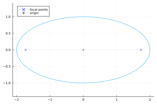
An ellipse is given by the equation:
\[\frac{x^2}{a^2} + \frac{y^2}{b^2} = 1 \label{eq:ellipse} \tag{3.2.1}\]Here is an ellipse with major axis $a=2$ and minor axis $b=1$:
It can be rotated and translated:
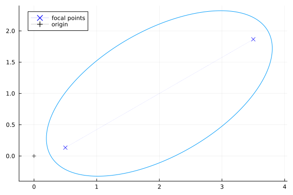
The equation for this general ellipse is:
\[\begin{align} x' &= x - x_0 \\ y' &= y - y_0 \\ x'' &= x'\cos\theta + y'\sin\theta \\ y'' &= y'\cos\theta - x'\sin\theta \\ \end{align} \label{eq:ellipse_general} \tag{3.2.2}\] \[\frac{(x'') ^2}{a^2} + \frac{(y'')^2}{b^2} = 1\]The promise of using ellipses is that, unlike polygons, the ellipse is represented by a single equation and all operations involving ellipses have formulas which can be evaluated directly in $O(1)$ time. The bottleneck instead comes from fitting the ellipse which is done using the mean and variance. Since these operations are $O(n)$, the whole process is $O(n)$.
The formulas require higher level mathematics than polygons. They involve quartic equations, more complex linear algebra, statistics and integral calculus.
Because the ellipse radii are based on standard deviations, they are less sensitive to outliers than convex hulls. However they share other drawbacks with polygons, such as no information given if the ellipses do not intersect. That is why this technique is still not recommended.
All these equations simplify to circles for $\sigma_x=\sigma_y$ and $\sigma_{xy}=0$ so that $a=b$.
Ellipses: fitting
The centre of the ellipse is given by the mean of the points. The orientation is given by the eigenvectors of the covariance matrix. The radii for the major and minor axis are given by the square root of the eigenvalues of the covariance matrix.
What are eigenvalues and eigenvectors? ⇩
Eigenvalues are a useful technique for working with matrices. They are the values $\lambda$ that together with the eigenvectors $v$ satisfy: $$ Av=\lambda v $$ For a square matrix $A$. That is, the whole matrix can be replaced with a single number. For example: $$ \begin{bmatrix} 3 & 2 \\ 1 & 2 \end{bmatrix} \begin{bmatrix} 2s \\ 1s \end{bmatrix} = 4 \begin{bmatrix} 2s \\ 1s \end{bmatrix} $$ For any value $s$. Here we have replaced the whole 2×2 matrix with a single number, 4. We could have also used the value 1 with its own eigenvector $(-1, 1)$. In general an $n\times n$ matrix will have $n$ eigenvalues where the trivial case of $\lambda=0$ and $v=\boldsymbol{0}$ is ignored.
This is an incredibly powerful form of dimension reduction. Conclusions about the whole matrix can be drawn from only the eigenvalues and eigenvectors. For example for the covariance matrix it is natural the two eigenvalues are the magnitudes of the greatest variances, because these are the two values that the whole matrix can be replaced with.
One might think the eigenvalue is restricted to only being useful for the particular eigenvector is it paired with. However because vectors can be made up as a sum of other vectors, any vector can be broken into $n$ distinct eigenvectors. So knowing the $n$ distinct eigenvalues is often enough.
This forms the basis for Principal Component Analysis (PCA).
The covariance matrix is:
\[C=\begin{bmatrix} \sigma_{x}^2 & \rho\sigma_{x}\sigma_{y} \\ \rho\sigma_{x}\sigma_{y} & \sigma_{y}^2 \\ \end{bmatrix} \label{eq:covariance} \tag{3.2.3}\]The eigenvalues are:
\[\begin{align} \lambda_{1,2} &= \frac{1}{2}\left(\sigma_{x}^2 + \sigma_{y}^2 \pm \sqrt{(\sigma_{x}^2-\sigma_{y}^2)^2 + 4\rho^2\sigma_{x}^2\sigma_{y}^2} \right) \\ \therefore a &= \sqrt{\lambda_1}, b =\sqrt{\lambda_2} \end{align} \label{eq:eigenvalues} \tag{3.2.4}\]With eigenvectors parallel to:
\[v_{1,2}=\begin{bmatrix} \lambda_{1} - \sigma_{y}^2 \\ \rho\sigma_{x}\sigma_{y} \end{bmatrix}s , \begin{bmatrix} \lambda_{2} - \sigma_{y}^2 \\ \rho\sigma_{x}\sigma_{y} \end{bmatrix}s \label{eq:eigenvectors} \tag{3.2.5}\]if $\rho\sigma_{x}\sigma_{y} \neq 0$ else the eigenvectors are along the $x$ and $y$ axis respectively. In practice these values are normalised so that $|v|=1$ when $s=1$.
The following shows the results with varying scales $s$:
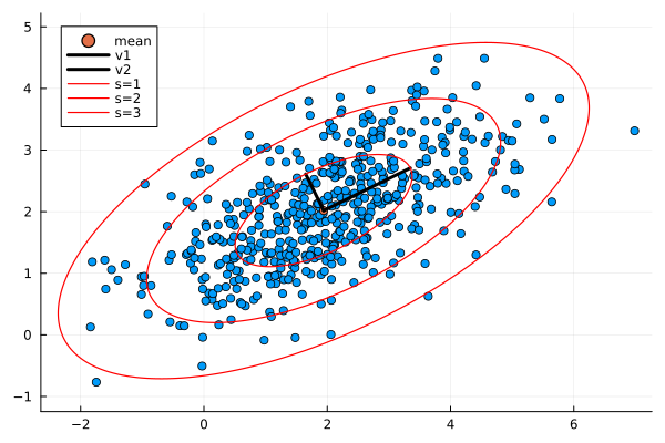
The scale $s$ represents a confidence interval. At first I thought that the eigenvalues were too small because for $s=1$ they only cover a small portion of points. However this is correct. The probability of a 2D point from the normal distribution lying within the ellipse for any scale is given by an exponential distribution:
\[p=1-e^{-\frac{1}{2}s^2} \label{eq:ellipse_prob} \tag{3.2.6}\]This is a Chi-squared distribution with 2 degrees of freedom. For intuition of why it is an exponential formula see this episode on a related problem by 3Blue1Brown. For more details see this question on stats.stackexchange.com and this paper: Algorithms For Confidence Circles and Ellipses, Wayne E. Hoover (1984).
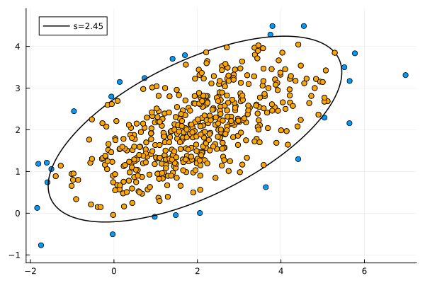
From equation $\ref{eq:ellipse_prob}$ approximately 39.3% of points will lie within the ellipse for $s=1$. We can invert this formula to solve for $s$ for any desired confidence interval:
\[s = \sqrt{-2\ln(1-p)} \tag{3.2.7}\]For a 95% confidence interval we need $s=2.4477…$. This is the result:
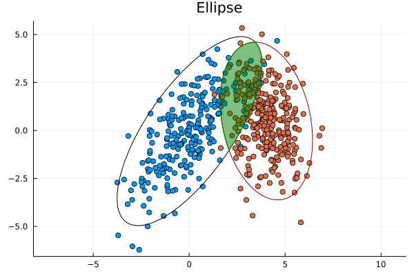
Ellipses: intersection
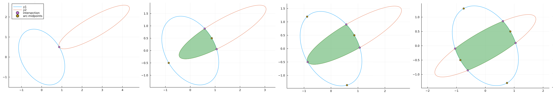
There are three special edge cases of ellipse-ellipse intersections: no intersection, one inside the other and identical ellipses on top of each other. These special cases can be tested using the extreme points of the ellipses. If they are far apart it can quickly be established that there is no intersection. Otherwise there are four distinct case for one to four points of intersection. Calculating these can require solving a quadratic, cubic or quartic equation.
Intersection points of ellipses ⇩
The following is a sketch of the algorithm to calculate the intersection points of two ellipses.
Equation $\ref{eq:ellipse_general}$ can be rearranged into the general conic section form: $$ a_0 + a_1x + a_2 y + a_3 x^2 + a_4 xy + a_5 y^2 = 0 $$ The second ellipse is then: $$ b_0 + b_1x + b_2 y + b_3 x^2 + b_4 xy + b_5 y^2 = 0 $$ Multiply each equation by the reciprocal of the co-efficient of the $y^2$ term and subtract one from the other to remove the $y^2$ term: $$ d_0 + d_1x + d_2 y + d_3 x^2 + d_4 xy = 0 \; ; \; d_i=\frac{a_i}{a_5}-\frac{b_i}{b_5} $$ Solve for $y$: $$ y = -\frac{d_0+d_1 x + d_3 x^2}{d_2 + d_4 x } \; ; \; d_2 \neq 0, d_4 \neq 0, x \neq -\frac{d_2}{d_4} $$ The edge cases where the denominator is zero (concentric ellipses / same ellipse horizontally translated) should be dealt with separately. Otherwise substitute back into the first ellipse equation: $$ f_0 + f_1 x + f_2 x^2 + f_3 x^3 + f_4 x^4 = 0 $$ where $f_i$ is some combination of $a_j$ and $d_k$ terms. (Have patience in collecting these terms.) Solve this quartic equation. If $f_0=0$, solving a cubic is sufficient.
Once the points of intersection are known the methods described in Calculating ellipse overlap areas by Gary B. Hughes and Mohcine Chraibi (2011) can be used to find the area of intersection. The two and three intersection point case require calculating two ellipse segments. The four case requires four ellipse segments and one inner quadrilateral. The arc-midpoints of the ellipse are used to determine which section of which ellipse is inside or outside the other.
How to compare scatter plots
Wasserstein metric
The Wasserstein metric is a statistical distance between two different distributions. It is symmetric, non-negative and obeys the triangle inequality. From Wikipedia:
Intuitively, if each distribution is viewed as a unit amount of earth (soil) piled on $M$, the metric is the minimum “cost” of turning one pile into the other, which is assumed to be the amount of earth that needs to be moved times the mean distance it has to be moved. This problem was first formalised by Gaspard Monge in 1781. Because of this analogy, the metric is known in computer science as the earth mover’s distance.
The mathematical definition is:
\[W_2(P_1, P_2) = \left( \inf\limits_{\pi \in \Pi(P_1, P_2)} \int\limits_{X\sim P_1, Y\sim P_2} ||X-Y||^2 d\pi(X,Y) \right)^{1/2} \tag{4.1} \label{eq:wasserstein}\]This states the metric $W_2$ is a scalar value that is the square root of the infimum (largest lower bound) of the integral (sum) of distances of points $X$ sampled from probability distribution $P_1$ to points $Y$ sampled from probability distribution $P_2$ over the joint probability distribution $\pi$ in the space $\Pi$.3
This definition should already indicate that the underlying mathematics is a level up in complexity from the previous sections. That said, the resulting equations are much simpler than the other methods.
The Hungarian method
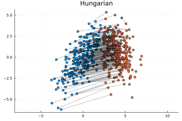
In the scatter plot above imagine moving the orange points onto the blue points. The constraint is a blue point can have only one orange point on top of it. Each orange point must be paired with its own blue point. The Wasserstein metric is then the smallest average distance once all orange points are moved out of all the possible ways of moving them.
This is a tricky problem to solve. A greedy algorithm will not suffice. What is good for a single point - e.g. moving it to the closet blue point to it - is not good for the overall population. That might also be the closest blue point for another point and therefore because it is taken that point will have to take its second closest point instead, but that has a knock-on effect too. Instead a better strategy is to assign the points on the outer edge first - try minimise these large costs first - and then slowly make your way to the centre.
A formal, optimal algorithm to solve this is the Hungarian Algorithm. It was designed to solve the assignment problem but this problem can easily be reframed as one. We consider assigning blue points to orange points where the distance between them is the cost.
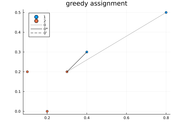
It is an interesting algorithm in part because it was designed to be done by hand. The algorithm is as follows:
- First do a greedy assignment. The other steps will iteratively improve this solution.
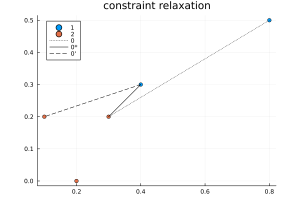
- Constraint relaxation: find the smallest cost that is not in use and open it up as a possible assignment.
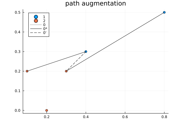
- Path augmentation: add this new smallest cost to solution, swapping old assignments to make room for it.
- Repeat steps 2 and/or 3 as many times as necessary until an optimal solution is found.
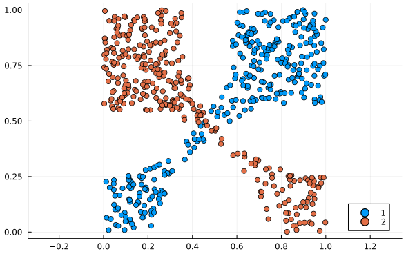
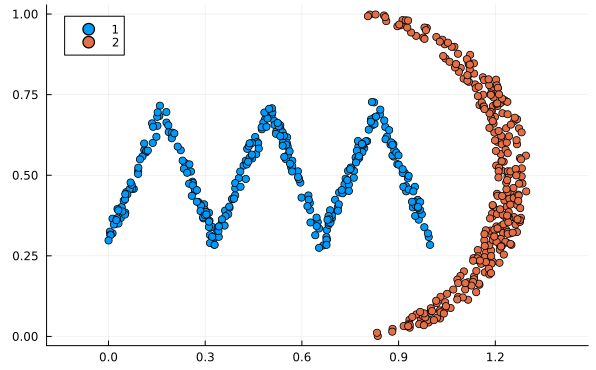
It runs in $O(n^4)$ time.4 While an impressive speed-up from the brute force $O(n!)\approx O(n^n)$, this still makes it the slowest algorithm reviewed here by a large margin. It compensates for this by being the most versatile. All the other methods assume the distributions are normal distributions and will fail if they’re not. Meanwhile this method works for all types of distributions. See these examples below:
Normal distribution approximation
If the data is from a normal distribution than the Hungarian solution can be approximated in $O(n)$ time. First find the means and covariance matrix (as with the ellipses). Then apply the following formula (proof in Givens & Short (1984)):
\[W_2(P_1, P_2)^2 = ||\mu_1 - \mu_2||^2 + \text{trace}\left(C_1 + C_2 -2 (C_1 C_2)^{1/2} \right) \tag{4.3.1} \label{eq:wasserstein_normal}\]The proof is very complex and requires a deep knowledge of linear algebra.
First they prove that the joint probability distribution of $Z=[X,Y]$ is itself a normal distribution with: $$ \mu = \begin{bmatrix} \mu_1 \\ \mu_2 \end{bmatrix}, \Sigma = \begin{bmatrix} C_1 & K \\ K^T & C_2 \end{bmatrix} $$ where $K$ is some $n\times n$ matrix, $\mu \in \mathbb{R}^{1\times 2n}$ and $\Sigma \in \mathbb{R}^{2n \times 2n}$.
Next note that: $$ \begin{align} Z^T A Z &= \begin{bmatrix} X^T & Y^T \end{bmatrix} \begin{bmatrix} I & -I \\ -I & I \end{bmatrix} \begin{bmatrix} X \\ Y \end{bmatrix} \\ &= X^T X + Y^T Y - X^T Y - Y^T X \\ &= (X - Y)^T (X - Y) \\ &= ||X - Y||^2 \end{align} $$ where $I$ is the $n\times n$ identity matrix. They use this with the trace trick for expectations of quadratic forms to evaluate the integral: $$ \begin{align} E[||X-Y||^2] &= E[Z^T A Z ] \\ &= \mu^T A \mu + \text{trace}(A\Sigma) \\ &= ||\mu_1 - \mu_2||^2 + \text{trace}(C_1 + C_2 - K - K^T) \end{align} $$
The problem is now one of finding a $K$ that minimises this equation subject to the constraint that $\Sigma$ remains a valid covariance matrix. This constraint is satisfied when $\Sigma$ is positive semi-definite: $$ x^T \Sigma x \geq 0 \; \text{for all } x \in R^{2n} $$ They then factorise $\Sigma$ using the Schur complement: $$ \Sigma = \begin{bmatrix} C_1^{1/2} & 0 \\ K^T C_1^{-1/2} & I \end{bmatrix} \begin{bmatrix} I & 0 \\ 0 & S \end{bmatrix} \begin{bmatrix} M_1^{1/2} & M_1^{-1/2}K \\ 0 & I \end{bmatrix} $$ Where $S=C_2 - K^T C_1^{-1}K$. From this they conclude that the constraint of $\Sigma$ being positive semi-definite is satisfied when $S$ is positive semi-definite. The problem is now reduced to: $$ \min_{K} \{ -2\text{trace}(K) \} \; \text{where } x^T (C_2 - K^T C_1^{-1}K)x \geq 0 $$ But this is still a difficult problem to solve. They solve it using eigen-decomposition (spectral decomposition) and Lagrange multipliers. This is well beyond the scope here. The result is that $K=(C_1^{1/2} C_2 C_1^{1/2})^{1/2}$.
Although they don't go further, because $C_1^{1/2} C_2 C_1^{1/2}=C_1^{-1/2}(C_1 C_2)C_1^{1/2}$ and $C_1 C_2$ are similar, they share the same eigenvalues and hence their square roots have the same trace. This is because $\text{trace}(A^{1/2})=\sum \lambda_i^{1/2}$ where $\lambda_i$ are the eigenvalues of $A$. See the Proof of symmetry card for more information.
The square root of a matrix $A$ is the matrix $A^{1/2}=B$ such that $BB=A$. There are several methods for finding it based on the properties of a matrix. For covariance matrices where $C=C^T$ the following formula can be used: $$ A^{1/2} = W D^{1/2} W^{-1} $$ where $W$ is a matrix of eigenvectors of $A$ and $D$ is the corresponding diagonal matrix of eigenvalues. The square root of a diagonal matrix is simply the square root of each of the elements along the diagonal.
Proof: $$ \begin{align} A^{1/2}A^{1/2} &= (W D^{1/2} W^{-1})(W D^{1/2} W^{-1}) \\ &= W D W^{-1} \\\ &= A \end{align} $$ Because $AW = WD$ from the definition of eigenvalues/eigenvectors.
Important things to note about this formula:
- It is composed of two terms. The first term is the distance between the means and the second term accounts for the difference in variance.
- If $C_1 = C_2$ than the metric is purely the distance between the means.
- If $C_2 = \boldsymbol{0}$ then the second term reduces to $\sigma_{1, x}^2 + \sigma_{1, y}^2$.
- In 1D it simplifies to: $(\mu_1 - \mu_2)^2 + \sigma_1^2 + \sigma_2^2 -2\sigma_1\sigma_2 = (\mu_1 - \mu_2)^2 + (\sigma_1 - \sigma_2)^2$.
- This formula is valid for distributions in 3D and beyond.
- It is symmetric in part due to the non-trivial equality $\text{trace}(C_1 C_2)^{1/2}=\text{trace}(C_2 C_1)^{1/2}$.
We want to prove that: $$ W_2(P_1, P_2)^2 = ||\mu_1 - \mu_2||^2 + \text{trace}\left(C_1 + C_2 -2 (C_1 C_2)^{1/2} \right) $$ is the same as: $$ W_2(P_2, P_1)^2 = ||\mu_2 - \mu_1||^2 + \text{trace}\left(C_2 + C_1 -2 (C_2 C_1)^{1/2} \right) $$
It is well known that $x^2=(-x)^2$ and that addition is commutative. The hard part is proving that: $$ \text{trace}(C_1 C_2)^{1/2}=\text{trace}(C_2 C_1)^{1/2} $$
The main prerequisite is the cyclic property of the trace: $\text{trace}(ABC)=\text{trace}(CAB)$.
Then for a diagonalizable matrix (no repeated eigenvalues) with eigenvectors $W$ and eigenvalues $\gamma$ in a diagonal matrix $D$: $$ \begin{align} AW &= WD \\ \therefore A &= WDW^{-1} \\ \therefore \text{trace}(A) &= \text{trace}(WDW^{-1}) \\ &= \text{trace}(W^{-1}WD) \\ &= \text{trace}(D) \\ &= \sum_i^n \gamma_i \\ \Rightarrow \text{trace}(A^{1/2})&=\text{trace}(WD^{1/2}W^{-1}) \\ &= \sum_i^n \gamma_i^{1/2} \end{align} $$
Also from the definition of eigenvalues: $$ \begin{align} C_1^{1/2}C_2 C_1^{1/2} v &= \lambda v \\ \times C_1^{1/2} \therefore C_1 C_2 (C_1^{1/2} v) &= \lambda (C_1^{1/2}v) \\ \therefore C_1 C_2 u &= \lambda u \; ; \; u =C_1^{1/2}v \\ \times C_2^{1/2} \therefore C_2^{1/2} C_1 C_2^{1/2} w &= \lambda w \; ; \; w =C_2^{1/2}u \\ \times C_2^{1/2} \therefore C_2 C_1 x &= \lambda x \; ; \; x =C_2^{1/2}w \end{align} $$ So $C_1^{1/2}C_2 C_1^{1/2}$, $C_2^{1/2} C_1 C_2^{1/2}$, $C_1 C_2$, $C_2 C_1$ share the same eigenvalues (but not eigenvectors). (The technical term is they are "similar" matrices.) Therefore their square roots have the same eigenvalues $\lambda_i^{1/2}$ and hence they have the same trace.
Some examples:
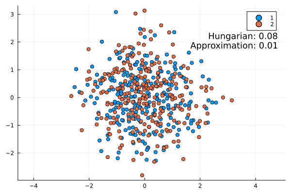
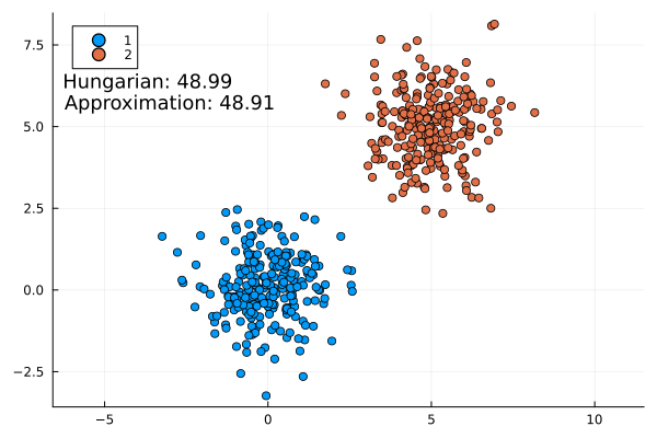
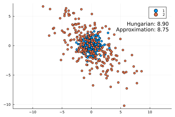
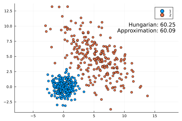
This approximation formula matches the actual result from the Hungarian method quite well. It is always slightly lower as expected (the infimum is the largest lower bound).
This really is the superior technique in terms of speed, ease, robustness, interpretation, and applicability. There is no need to consider any other method to compare scatter plots.
Conclusion
This has been a long post for a simple conclusion: equation $\ref{eq:wasserstein_normal}$ can be applied in most scenarios to measure the difference between scatter plots. This formula can be implemented in a single line with a standard linear algebra package. However this post was not just about the conclusion. It was also about the journey in exploring different solutions and comparing visual approaches with a statistical one.
I hope this post has given insight into problems like this. Sometimes it is better to follow established practices rather than reinvent the wheel.
Some humility is important too. It is frustrating to hear the argument that equation $\ref{eq:wasserstein_normal}$ is too complex in favour of the whole polygon approach. The one is a maths formula; the other is a whole multi-step iterative-based algorithm with many failure points. This work justified my initial thoughts. The polygon method required over 1000 lines in code and extensive testing; the formula only 30.5
When creating the widget at the start, I considered adding all the methods. However - unlike Julia - JavaScript is not a numerical programming language. While the Wasserstein formula itself is still short there are almost 190 lines of code for the basic linear algebra. The polygon and ellipse methods would probably have similar increases in code. As in the original use case I decided they were way too much effort.
Code analysis
This is a detailed breakdown of the table from the introduction.
| Method | Algorithm | Time Complexity | Source / test LOC | Reference |
|---|---|---|---|---|
| Polygon (410 / 640 LOC) | Convex hull: Gift Wrapping | $O(nh)$ | 70 / 80 |
Wikipedia |
| Intersection points of convex polygons | $O(n+m)$ | 100 / 280 | O'Rourke et. al. 1982 | |
| Intersect segments | $O(1)$ | 100 / 50 | ||
| Orientation of segments | $O(1)$ | 40 / 0 | GeeksForGeeks | |
| Area polygon: shoelace formula | $O(n)$ | 30 / 50 | Wikipedia | |
| Point in polygon | $O(n)$ | 70 / 180 | Galetzka and Glauner 2017 | |
| Ellipses (490 / 350 LOC) | 2x2 eigenvalues | $O(1)$ | 30 / 0 | |
| Solve quadratic / cubic / quartic | $O(1)$ | 100 / 70 | Wikipedia | |
| Point in ellipse | $O(1)$ | 50 / 0 | ||
| Intersection points of ellipses | $O(1)$ | 130 / 210 | ||
| Areas of intersection of ellipses | $O(1)$ | 180 / 70 | Hughes and Chraibi 20211 | |
| Hungarian (410 / 370 LOC) | Distance matrix | $O(n^2)$ | 10 / 0 | |
| Munkres method | $O(n^4)$ | 400 / 370 | Duke University | |
| Wasserstein (30 / 0) LOC | Normal distribution Wasserstein metric | $O(1)$ | 30 / 0 | Wikipedia |
-
Lines of Code is a controversial metric that can be very misleading. It can be easily gamed. For example by squeezing many characters on one line, leaving out comments, documentation or empty spaces and neglecting to count packages or tests as part of the metric. It can penalise more efficient code. For example, preallocation of objects can speed up code. That said, it can be a useful approximation of the amount of effort that goes in to code in lieu of more meaningful but abstract metrics. This is the reason I have chosen to use it. Here a line is defined as “140 characters or less”. All comments, documentation and blank lines are included in the counts - these are important for humans, if not computers. Source code and test code are reported separately. Packages are only included in the count if they do not come preinstalled (so not in
Base.jl). The final number is rounded to the nearest nice number - this is a fuzzy metric after all. ↩ -
Technically the perimeter of an ellipse requires an infinite sum. However there are very good approximation formulas. ↩
-
The infimum is the largest lower bound. A lower bound on the metric is 0 but to be useful it should be as close as possible to the minimum value of the integral. Ideally the lower bound is the minimum value. In the discrete case the infimum is the minimum. For the normal distribution formula you would need an infinite number of points to accurately model it and find a minimum. The infimum is the value that this minimum asymptotically tends to. ↩
-
Some sources claim it runs in $O(n^3)$ time. This is not my assessment. The worst case is $n^2$ runs of the outer loop and the constraint relaxation step takes $O(n^2)$ time. This is overall $O(n^4)$. In general anywhere from 0 to $n^2$ loops are required and so executions will run in $O(n^k)$ time where $2 \leq k \leq 4$. ↩
-
Other lines of code are for: comments, documentation, calculating the means and variances and handling numerical errors. ↩