A recent paper caused a stir in the machine learning world. It claimed that a combination of GZip and k-Nearest Neighbours could beat transformers in classification tasks. Here I implement that method in Julia and explore results for two datasets, one of which was used in the original paper. The method has clear merits but questions have been raised about the accuracy method reported in the original paper. Because of this and other concerns, I don’t see it as a better alternative to the classic TF-IDF and logistic regression combination.
Table of Contents
Introduction
The paper “Low-Resource” Text Classification: A Parameter-Free Classification Method with Compressors by Jiang et al (2023) presents an interesting method for text classification. It is based on the insight that compressing two pieces of similar text will result in less bytes than compressing two pieces of dissimilar text. Any text compressor can be used. The authors chose GZip because it is a “simple compressor”.
This is mathematically captured as follows: denote $C(x)$ as the length of bytes of the compressed text $x$ and $xy$ as the concatenation of texts $x$ and $y$ with a space. Then define the Normalized Compression Distance (NCD) as:
\[\text{NCD}(x,y) = \frac{C(xy)-\min\{C(x), C(y)\}}{\max\{C(x), C(y)\}}\]The label of $x$ can be found as the label of a reference text $y$ which minimises $NCD(x, y)$. A more robust method is to use the k-Nearest Neighbours technique: the label of $x$ is the most common label amongst the $k$ reference texts with the $k$ lowest NCD scores.
The authors claim this method is simple and effective. The paper compares it to other machine learning techniques including transformers with millions of parameters. They test it across 12 datasets and achieve accuracies up to 97%. In many cases it beats or comes close to the accuracies achieved by the other machine learning methods.
Here I explore this technique in detail for a single data set, AG News. My findings are less complimentary. After re-evaluating the accuracy more fairly, this method falls in the bottom half of the techniques/models in the table. Further, the implementation itself is very slow in both setup and inference. As far as “low resource” techniques go, I find that it does not beat the classic Term Frequency - Inverse Document Frequency + Logistic Regression (TF-IDF + LR) combination in accuracy, practicality or interpretability.
Code
This technique is simple enough to be captured in a few lines of code. Here are the original 14 lines of Python from the paper that have been proudly paraded on social media:
import gzip
import numpy as np
for (x1, _) in test_set:
  Cx1 = len(gzip.compress(x1.encode()))
  distance_from_x1 = []
  for (x2, _) in training_set:
    Cx2 = len(gzip.compress(x2.encode())
    x1x2 = " ".join ([x1, x2 ])
    Cx1x2 = len(gzip.compress (x1x2.encode())
    ncd = (Cx1x2 - min(Cx1, Cx2)) / max(Cx1, Cx2)
    distance_from_x1.append(ncd)
sorted_idx = np.argsort (np.array (distance_from_x1))
top_k_class = training_set[sorted_idx[:k], 1]
predict_class = max(set(top_k_class),key=top_k_class.count)
This is not the code that the paper uses. That can be found here. But it is impressive that it can be condensed into a few lines of code.
I’d like to present a Julia version of this in 23 lines of code:
using CodecZlib
using StatsBase
function knn_gzip_classification(
    text::AbstractString, ref_data::Vector{<:AbstractString}, labels::Vector; k::Int=2)
    distances = make_distance_vector(text, ref_data)
    sorted_indices = sortperm(distances)
    top_labels = labels[sorted_indices[1:k]]
    frequencies = countmap(top_labels)
    findmax(frequencies)[2] # always returns the first maximal element
end
function make_distance_vector(text::AbstractString, ref_data::Vector{<:AbstractString})
    distances = Vector{Float64}(undef, length(ref_data))
    length1 = length(transcode(GzipCompressor, text))
    for (i, x2) in enumerate(ref_data)
        distances[i] = normalised_compression_distance(text, length1, x2)
    end
    distances
end
function normalised_compression_distance(text1::AbstractString, length1::Int, text2::AbstractString)
    length2 = length(transcode(GzipCompressor, text2))
    length12 = length(transcode(GzipCompressor, text1 * " " * text2))
    (length12 - min(length1, length2)) / max(length1, length2)
end
Other than the necessary differences between the languages, there are two major style differences with my Julia version:
- I have three separate functions instead of one big function. I think this is important, not only because Julia is a functional language, but for general readability and compiler optimisation. It is trivially easy to reduce it further by 5 lines1 in the single minded pursuit of a lower line count but I do not think it is worth it.
- I have not included the outer loop which loops over the test set. It is unusual that the source code does this. The norm is to have a reusable function which can be used in conjunction with multiple tests rather than code which integrates testing and functionality.
This is more than just pedantics. It is worrying that the actual codebase also mixed the test loop with the inference loop. This obfuscated a biased accuracy calculation in the case of ties. Ken Schutte raised this concern in a post and addressed further issues in a second post. I highly recommend reading Schutte’s post before continuing, although the next section will give a brief overview. You can also see the main author’s response on this GitHub issue.
For the full code see my repository at github.com/LiorSinai/CompressorClassification.jl.
Tie breaking
A problem with kNN is tie breaking: what happens if there is no “most common” label because multiple labels share the same (maximum) frequency? This is especially relevant for $k=2$ which was the value of $k$ used in the paper. It is very easy for the top 2 reference samples to have different labels and hence there will be a tie.
The original codebase has the option to do tie breaking randomly. This is a decent strategy. However the results are reported without tie breaking. Instead predictions are marked as correct if either label is correct.
In order to replicate this strategy, I created a separate method called knn_classification_multi which returns type Vector{Int64} instead of type Int64. It as follows:
function knn_classification_multi(
    distances::Vector{Float64}, labels::Vector
    ; k::Int=2)
    sorted_indices = sortperm(distances)
    top_labels = labels[sorted_indices[1:k]]
    most_common_classes = get_most_common_neighbours(top_labels)
    most_common_classes
end

function get_most_common_neighbours(labels::Vector)
    frequencies = countmap(labels)
    max_freq = maximum(values(frequencies))
    collect(keys(filter(pair->pair[2] == max_freq, frequencies)))
end
The accuracy function can then be written as:
accuracy(y_pred::Vector{<:Vector}, y_test::Vector) =
    count(yy -> yy[2] in yy[1], zip(y_pred, y_test)) / length(y_test)
This is the “top-2” accuracy that Ken Schutte refers to in his work. I think the biggest issue with this strategy is that it is not used for the other techniques reviewed in the paper. That is unfair and gives this technique an edge over the others. The next section AG News will show exactly how significant this edge is.
This is the standard accuracy calculation for comparison:
accuracy(y_pred::Vector, y_test::Vector) =
    count(yy -> yy[2] == yy[1], zip(y_pred, y_test)) / length(y_test)
Or equivalently:
accuracy(y_pred::Vector, y_test::Vector) = mean(y_pred .== y_test)I have also implemented three tie breaking strategies:
- random: randomly select a label with uniform probability.
- decrement: decrement $k$ and recalculate scores until the tie is broken or $k=1$.
- min total (weighted): select the most common class with the lowest total NCD. Another way to think of this is instead of each sample having a vote of $\text{weight}=1$, each sample has a vote of $\text{weight}=\text{NCD}$.
The “decrement” and “min total” strategy will mostly align but not always. These strategies are both mostly deterministic.2
AG News
The AG News classification dataset is a dataset of 120,000 news headlines with an additional 7,600 test headlines. They are evenly split into 4 catagories: World (0), Sports (1), Business (2) and Sci/Tech (3). Here are examples:
| label | text |
|---|---|
| World | 2 Aid Workers Are Freed After 3 Weeks in Captivity Two Italian aid workers kidnapped 21 days ago in an audacious daylight raid were freed Tuesday, the prime minister of Italy announced. |
| Sports | For starters, Eli makes case CHARLOTTE - Kurt Warner may still be the favorite to start the regular-season opener for the Giants. But Eli Manning isn #39;t making Tom Coughlin #39;s decision very easy. |
| Business | Eyetech Pins Its Hopes (and Shares) on New Drug An experimental eye disease drug has been a boon to Eyetech Pharmaceuticals. But as the drug nears approval, many doctors are questioning its effectiveness. |
| Sci/Tech | Hewlett-Packard takes a new approach to software The company extends a deal with open-source Java software maker JBoss in an effort to compete with IBM. |
Creating a 120,000×7,600 distance matrix for this dataset took 3 hours 13 minutes on a 2.30 GHz processor with 16 threads with 16GB of RAM. The matrix was stored in an Arrow file with a size of 6.8GB.3 The paper claimed to have done this in 30 minutes with an 8 core CPU.
This is a significant upfront computational cost for this technique and already a good reason to be hesitant of using it.
The accuracy in the paper reported for AG News is 93.7%. I was able to replicate this with the above knn_classification_multi method.
Once I had done that, I had other questions:
- What is the influence of the neighbourhood size $k$?
- What is the influence of different tie breaking strategies?
- What is the influence of the total number of reference samples? That is, the training data size?
- How does the practical implementation compare to other methods? For example, inference times and object sizes?
The next few sections will answer these.
Neighbourhood size

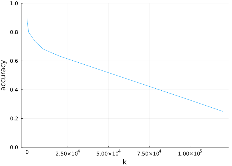
It is best to keep the neighbourhood size small. Multiple samples do make the estimate more robust but this reaches an optimum very quickly. For this dataset it is $k\approx 10$. After this more samples only add noise. The method eventually dissolves into pure guessing at $k=N$.
Tie breaking strategies
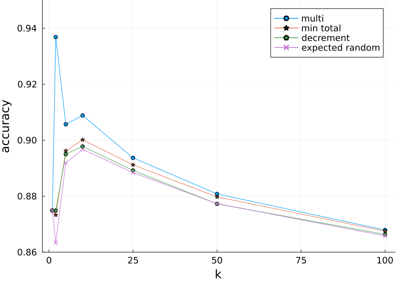
Based on the previous results, we only need to explore $1\leq k \leq 100$.

Here the “random” accuracy is given as the expected random accuracy.
That is, the labels are calculated using the knn_classification_multi method and then an even $\tfrac{1}{k}$ chance is given to selecting the correct label. For example for $k=2$ there are 6003 predictions with the correct most common label and another 1253 ties of which 1117 contain the correct answer.
If all the ties are broken correctly the accuracy will be 7120/7600=93.7%.
However it is more likely that only half will be, so the expected accuracy is 6561.5/7600=86.3%.
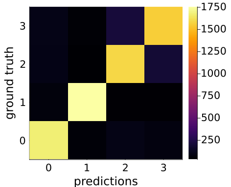
The accuracy of 93.7% is an outlier in this graph. We have the alternatives of this either being a fluke or something special is happening in the dataset with $k=2$. (This method is parameter free so we can safely rule out model artifacts.) In this case it is actually the latter. The confusion matrix for random guessing helps with further insight:

So confusion is usually only between the Business (2) and Sci/Tech (3) classes. Here are some samples that were confused:
| Label | Predicted | Text |
|---|---|---|
| Business | Sci/Tech | AOL, E-Mail Companies Sue Spammers The nation #39;s largest e-mail providers today filed a new round of lawsuits against Internet spammers allegedly responsible for shoveling millions of junk e-mail messages into computer users #39; in-boxes and their instant messaging screens. |
| Business | Sci/Tech | HP to tempt holiday shoppers with sights and sounds The computer-hardware giant, best known for products such as PCs and printers, on Friday laid out its plan to become a brand-name in consumer electronics products such as flat-screen TVs, music players and the devices that move content between them. |
| Sci/Tech | Business | Microsoft Brings TV to Xbox October 14, 2004 - Microsoft is set to release its Windows Media Center Extender for Xbox mid-November. The device will allow you to view recorded and downloaded media content stored on your PC via your Xbox. |
| Sci/Tech | Business | Update: Intel shelves plans for 4GHz Pentium 4 Intel Corp. has confirmed its near-term plans for its desktop processors before it reaches the multicore era. The company will not release a 4GHz version of its flagship Pentium 4 product, having decided instead to realign its engineers around the company's new design priorities, an Intel spokesman said Thursday. |
All four samples relate to announcements by technology companies - AOL, HP, Microsoft and Intel - but the first two are Business headlines and the last two Sci/Tech headlines. The first two rows include technology terms like “internet” and “computer”. The last two include business terms like “release”, “company” and “spokesman”. Its easy to see how the model can confuse these.
We can conclude that the outlier is more an indicator of problems in the data than of hidden intelligence in the method. It is not representative of this graph yet it is the only number in it that is presented in the paper!
By using this “top-2” outlier this method gains a non-trivial boost in accuracy in the paper. It places at 3/14 of the models investigated. If instead random accuracy was used it would place at 11/14. Or if the peak at 90.0% was used, obtained with $k=10$ and the min total tie breaking strategy, it would still only place at 8/14.
I am curious if this phenomenon holds for other datasets used in the paper. I have not investigated further.
Moving on from this issue, the best tie breaking strategy is consistently the min total except for $k=2$. It also has the advantages of being deterministic and quantifiable.
Reference sample size
The next question is, how does the sample reference size affect the accuracy? The paper benefits from large training datasets which were collected for machine learning algorithms that are very data hungry. However this method is parameter free and theoretically can work with much less data. A smaller dataset would result in reduced accuracy but it would also result in quicker distance matrix construction times, smaller distance matrices and faster inference. This tradeoff might be worth it.
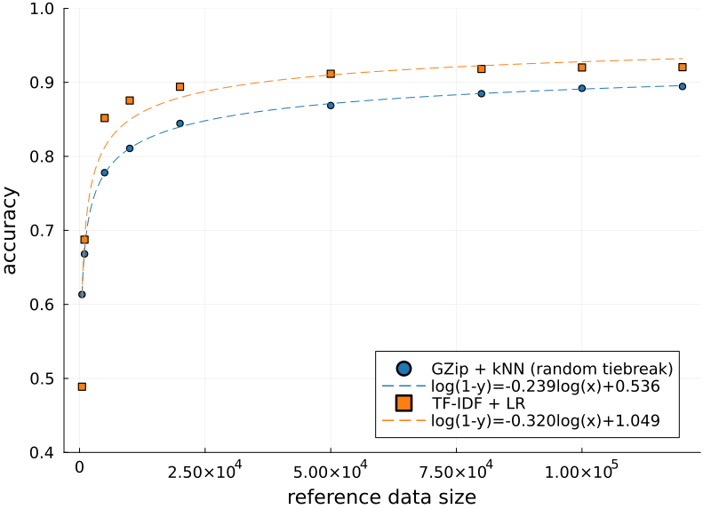
To test this, I randomly took $n$ training examples and used these to calculate the accuracies. These could be sampled directly from the existing distance matrix because all the rows are independent of each other. I did the same for the TF-IDF + LR model, training each logistic regression model on 10 epochs. The resulting graph is arguably the most condemning so far:

The curves are fit to the following equation (source):4
\[\begin{align} \epsilon &= a n^{-\alpha} + \epsilon_0 = e^c n^b + 0 \\ \implies \log(\epsilon) &= c + b \log(n) \end{align}\]where $\epsilon$ is the error, $1-\epsilon$ is the accuracy and $n$ is the training/reference data size. The intrinsic error $\epsilon_0$ is assumed zero for simplicity.
Starting from $n=1000$ the TF-IDF + LR method takes over and maintains the highest accuracy. The top accuracy obtained was 92%.
Practical considerations
The paper only compares the models based on accuracy. For practical purposes it is also useful to compare on other metrics like object sizes and training and inference times. I compared the GZip + kNN method with TF-IDF + LR and with a 330,000 parameter transformer. The results can be seen in the table:
| Factor | GZip + kNN | Transformer | TF-IDF + LR |
|---|---|---|---|
| Parameters | 0 | 331,949 | 74,104 |
| Model file size (MB) | 0 | 1.6 | 0.4 |
| Transformed data size (MB) | 6963 | 2.9 | 2.7 |
| Training time (min) | 195 | 30 | 1.6 |
| Inference time (sec/7600 samples) | 120 | 5.1 | 0.3 |
| Test accuracy (%) | 90.0 | 91.1 | 92.1 |
Further details:
- The code is all written in Julia. You can see my repositories at CompressorClassification.jl, TransformersLite.jl and TermFrequencyInverseDocumentFrequency.jl.
- Transformer details:
- Text preprocessing: lowercase, remove unicode characters and punctuation.
- Vocabulary size: 9,969. All 2 letter words with a document frequency greater than 28.
- Embedding dimension: 32.
- Encoder stacks: 1.
- Training epochs: 10.
- TF-IDF + LR details:
- Text preprocessing: lowercase, remove unicode characters and punctuation.
- Vocabulary size: 18,525. All 2 letter words with a document frequency greater than 9.
- Training epochs: 10.
- The accuracy of 92.1% is higher than the value of 89.8% reported for this method in the paper.
This GZip + kNN method does very poorly in this table. Compared to TF-IDF + LR it is 100 times slower for training and inference and it requires 2500 times more space. Even compared to the transformer it is slow, taking 6.5 times longer to generate the distance matrix than to fully train the 330,000 parameter model from scratch. All this for the method with the lowest accuracy in this table.
Interpretability and explainability are also important in practical use cases:
- TF-IDF + LR is very easy to interpret: there is one weight per word per class (and the bias terms). A ranking of weights shows the most important words per class.
- Transformers are more complex but some effort has been to understand their many weights.
- The GZip part is the main black box in the GZip + kNN technique. Without diving into its complexities there is no obvious way I know of to understand why it compresses some samples more.
For now, I think GZip + kNN is the least explainable.
Amazon Reviews Multi
I briefly investigated performance on another data set, Amazon Reviews Multi. This is a sentiment analysis task to predict Stars on Amazon reviews with 1 being very negative and 5 being very positive. It has 200,000 English language training samples along with 5,000 test samples. The accuracy achieved here was 41.9%. This was below a 51.5% accuracy achieved with TF-IDF + LR and a 50.9% accuracy achieved with a 225,00 parameter transformer.
A simpler task is binary classification. All 1 and 2 stars are set as negative (0) and all 4 and 5 stars are set as positive (1). The 3 star samples are dropped. The accuracy achieved here was 79.4% for $k=9$ compared to 89.6% with the TF-IDF + LR model and 86.9% with a 225,000 parameter transformer.
It should be noted that in the binary case there is a straight forward method to avoid ties: choose odd $k\geq3$. Then there will always be at least one sample breaking the two-way tie.
Unfortunately there is no magic $k$ like this in the general case.
Conclusion
The simplicity of compressor classification caught my attention but it failed to live up to the hype on social media. In reality it is clunky to implement and frustratingly slow. Older techniques can be done 100 times quicker with greater accuracy. As for the paper itself, the utilisation and defense of an unfair accuracy method seriously detracts from its authenticity.
That said, I hope this article does not come across as too negative. The method is novel, based on sound principles and it does work. While it is not very practical now it could lead to other interesting research in the future.
-
Lines 10, 11, 17, 18 and 19. ↩
-
There is a small amount of randomness remaining from the sorting.
For example, if $k=2$ is used but the top 3 samples all have the same NCD score then uncontrolled factors will influence which 2 samples are chosen.
Shared scores are highly prevalent. For example for AG News, on average only 2.4% of each column of the distance matrix is unique and the rest are repeat values. ↩
-
With GZip this matrix can be compressed from 6.79 GB to 1.75 GB. Further compression is surely possible since 2.4% of the matrix is unique and the rest is repeat values. ↩
-
Fitting a linear regression curve is very easy and I worry not well known enough. The function is:
function fit_linear_regression(x::Vector, y::Vector)
    X = hcat(x, ones(length(x)))
    b = X \ y
    b
end
where the
\operator will calculate $X^+y$ which makes use of the Moore–Penrose inverse $X^+=(X^T X)^{-1}X^T$ and is the optimal solution to minimise the mean squared error . For the logistic regression curve, pass in(log.(x), log.(y)). ↩