DeepSeek's Multi-Head Latent Attention

A deep dive into DeepSeek’s Multi-Head Latent Attention, including the mathematics and implementation details. The layer is recreated in Julia using Flux.jl.

See also previous posts on transformers:

• Transformers from first principles in Julia.
• Generative transformer from first principles in Julia.

All code available at github.com/LiorSinai/TransformersLite.jl/tree/feature/mla.

Table of Contents

1 Introduction

In January 2025, DeepSeek unveiled their new DeepSeek-V3 and DeepSeek R1 models. It took the world by storm. Users were impressed with its abilities on top of their claims that is was up to 50× more efficient to train and run than their competitors.

They also released multiple papers (DeepSeek-V2, DeepSeek-V3, DeepSeek-R1) with an impressive array of new techniques across the whole machine learning pipeline, from high level theory to intricate implementation details. Most of it built on existing ideas in innovative ways. They include:

• Theory
  • Multi-Head Latent Attention: compress vectors during attention, which reduces computation and during inference reduces cache size.
  • DeepSeekMoE: segmented and isolated mixture of experts.
  • Multi-token prediction.
  • Reinforcement learning with Group Relative Policy Optimization but without supervised data.
  • Improved chain-of-thought reasoning.
• Implementation
  • DualPipe: accelerate training by overlapping forward and backward computation communication phases.
  • Exponential moving average on the CPU.
  • Mixed precision floating point numbers during training. FP8 and FP32 are used.
  • Low-precision storage and communication.

The aim of this post is to explore one of these ideas in depth, namely Multi-Head Latent Attention (MLA), which has the primary aim of reducing the cache size but the compression involved also gives a decent performance boost.

As we will see, MLA actually combines 3 ideas:

1. Attention and multi-head attention from Attention is all you need (2017).
2. KV Caching.
3. Low-Rank Adaption matrices (LoRA) from LoRA: Low-Rank Adaptation of Large Language Models (2021).

This article assumes you have some exposure to these techniques already.

DeepSeek also adds two enhancements:

1. Weight absorption.
2. Decoupled rotary position embeddings (RoPE) from RoFormer: Enhanced Transformer with Rotary Position Embedding (2021).

While the DeepSeek paper only speaks good of these, they complicate the mathematics and require specialised optimised code to see real performance gains.

The original source code is written in Python with the PyTorch machine learning framework. However, my favourite language is Julia and continuing with my previous posts on transformers, all the code here is written in Julia using the Flux.jl machine learning framework. The mathematics therefore follows Julia’s columnar major format and not Python’s row major format. In this format each column represents a single sample. The second dimension is sequence length and all remaining dimensions represent batches.

2 KV Caching

2.1 Theory

There is an inefficiency in using transformers for generation. In classification use cases, the model only needs to calculate attention over the input sentence once (per layer) before making its prediction. But in text generation, it needs to recalculate it over the entire sentence. One analogy I read is that this is like having to reread the entire sentence so far in order to produce the next word and then rereading again to produce the next word, and so on.

In mathematical terms, this requires computing the attention between the first token and itself, between the first two tokens, between the first 3 tokens and so on until it’s between all the tokens, and repeating this whole process each time for every new token. This was the case for the generator I made based on Andrej Karpathy’s Zero to Hero course.

It would be better to have a “memory” of what has been generated so far. This is where the KV cache comes in, for Key-Value cache. We can store the previous keys and values and use them to calculate the new attention value. This will give the exact same value as recalculating the entire attention.

Here is a mathematical proof. For a visual interpretation, please see João Lages’ excellent article.

The attention equation is

where

where $X \in \mathbb{R}^{d\times n \times B}$ and $W^K, W^Q, W^V \in \mathbb{R}^{d_hH \times d}$.

Focusing on one head in one batch with dimension $d_h$, the input matrix $X$ is split into the first $n-1$ columns and the $n$th column. The first multiplication can then be written as (dimensional analysis on right):¹

Looking at the final line, the first $(n-1)$ columns of the query can be safely dropped without affecting the $n$th column. (We would do this anyway in generation.) The $n$th column only depends on $K_{1:n-1}$, $K_n$ and $Q_n$. Of these, $K_{1:n-1}$ will come from the cache and the other two will be calculated from $X_n$.

Similarly for the next multiplication we have ($Z=\text{softmax}(S)$):

However, we said we are dropping the first $(n-1)$ columns. Without them only the $n$th column is calculated. Hence we have:

which depends on $V_{1:n-1}$, which will come from the cache, and $V_n$, which will be calculated from $X_n$.

There will be two caches each with size $d_h H \times N \times B$ for $H$ heads, a maximum sequence length of $N$ and a maximum batch size of $B$. The total cache size can grow very large for large transformers with many multi-head attention layers. The primary aim of MLA is to reduce the size of this cache. That will be covered in the next section.

2.2 Code

Building on my code in TransformersLite.jl, it is straightforward to create a new MultiHeadAttentionKVCache layer with two caches:

struct MultiHeadAttentionKVCache{
    Q<:Dense, K<:Dense, V<:Dense, O<:Dense, C<:Array{T, 3}  where T
    }
    nhead::Int
    denseQ::Q
    denseK::K
    denseV::V
    denseO::O
    cache_k::C
    cache_v::C
end

Flux.@layer trainable=(denseQ, denseK, denseV, denseO)

The forward pass calculates the current q, k and v values from the input and gets the rest from the cache. It then continues without any additional modifications from the original code:

function (mha::MultiHeadAttentionKVCache)(
    query::A3, key::A3, value::A3
    ; start_pos::Int=1, use_cache::Bool=true, kwargs...
    ) where {T, A3 <: AbstractArray{T, 3}}
    q = mha.denseQ(query) # size(q) == (dh, 1, B)
    k = mha.denseK(key)
    v = mha.denseV(value) # size(k) == size(v) == (dh, 1, B)
    if use_cache
        dim, seq_length, batch_dim = size(query)
        end_pos = start_pos + seq_length - 1
        mha.cache_k[:, start_pos:end_pos, 1:batch_dim] = k
        mha.cache_v[:, start_pos:end_pos, 1:batch_dim] = v
        K = mha.cache_k[:, 1:end_pos, 1:batch_dim]
        V = mha.cache_v[:, 1:end_pos, 1:batch_dim]
    else
        K = k
        V = v
    end
    A, scores = multi_head_scaled_dot_attention(mha.nhead, q, K, V; kwargs...)
    mha.denseO(A), scores
end

Here is a small example of it in action. (For the full code, see test/MultiHeadAttention.jl.)

Create the layer and inputs:

using TransformersLite
using TransformersLite: MultiHeadAttention, MultiHeadAttentionKVCache
using TransformersLite: make_causal_mask, clone_add_kv_cache
nhead, dim_model, dim_out = 4, 32, 13
mha = MultiHeadAttention(nhead, dim_model, dim_out) 
mha = clone_add_kv_cache(mha, 64, 8)
X = randn(Float32, 32, 10, 5)

Fill the cache:

mask = make_causal_mask(ones(10, 10))
A, scores = mha(X, X, X; mask=mask, start_pos=1, use_cache=true)
size(A) # (13, 10, 5)
size(scores) # (10, 10, 4, 5)

Use the cache with a new vector:

x = randn(Float32, 32, 1, 5)
mask = repeat([true], inner=(11, 1))
Ax, scoresx = mha(x, x, x; mask=mask, start_pos=11, use_cache=true)
size(Ax) # (13, 1, 5)
size(scoresx) # (11, 1, 4, 5)

Compare without the cache:

Xx = cat(X, x, dims=2)
mask = make_causal_mask(ones(11, 11))
AXx, scoresXx = mha(Xx, Xx, Xx; mask=mask, start_pos=1, use_cache=false)
isapprox(AXx[:, end, :], Ax[:, end, :]) # true

3 Multi-Head Latent Attention

3.1 C cache

We’ve seen that the KV cache has size $2d_h H \times N \times B$ elements per multi-head attention layer. (Each element is 1-4 bytes depending if FP8, FP16 or FP32 is used.) The aim of MLA is to reduce this, specifically to $d_c \times N \times B$ elements per multi-head attention layer. Therefore we will choose $d_c < 2d_h H$.

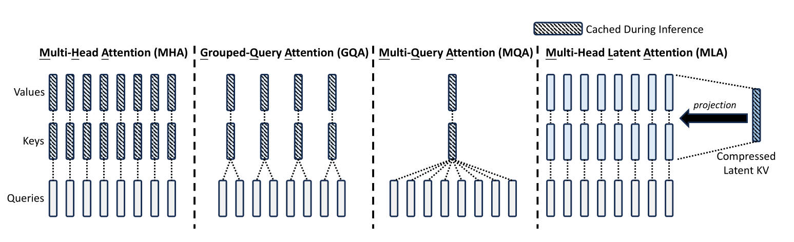
DeepSeek’s innovation is to introduce a weight matrix $W^{DKV} \in \mathbb{R}^{d_c\times d}$ to compress the input $X \in \mathbb{R}^{d\times n}$ to a lower rank matrix $C^{KV} \in \mathbb{R}^{d_c \times n}$. This $C^{KV}$ matrix is then stored in the cache. Then two other weight matrices $W^{UK}$ and $W^{UV} \in \mathbb{R}^{d_h H\times d_c}$ uncompress the same $C^{KV}$ matrix to the key $K$ and value $V$ respectively. The above figure shows this visually.

The KV cache is now replaced with a $C^{KV}$ cache of size $d_c \times N \times B$. DeepSeek theorises that this compression also results in a regularization effect that improves performance. This is supported by other LoRA research. However, the lossy compression might instead adversely affect quality. DeepSeek provides no evidence towards either claim.

The compression also results in a significant performance boost which DeepSeek strangely does not mention in their paper. Note that in MLA there are three matrix multiplications to perform comprising of $2(2d_hH + d)d_c nB$ scalar operations instead of two matrix multiplications comprising of $4(d_h H)d n B$ operations in MHA.² With the standard $d = d_h H$ and a compression ratio $r=\tfrac{d_h H}{d_c}$, the ratio of operations with MLA compared to MHA is $\tfrac{3}{2r}$. Therefore this requires only $r>1.5$ for a performance boost too. The only performance penalty is the memory required for the $n$th $c^{KV}_n$ vector before it is transferred to the cache, which is $d_c \times 1 \times B$.

DeepSeek-V3 uses $d_h = 128$, $H=128$ and $d_c=4 d_h = 512$ which means it has a compression ratio of $32$ and a 20× speed up!

To reduce the activation memory during training, DeepSeek also applies the same strategy to the query:

DeepSeek give further enhancements to this which will be described shortly. They also apply layer normalisation to $C^Q$ and $C^{KV}$ which I will ignore in this article. For now, lets see this basic version of MLA in action.

3.2 Code

First create a struct similar to the MultiHeadAttentionKVCache layer.

struct MultiHeadLatentAttention{D1<:Dense, D2<:Dense, A<:AbstractArray{T, 3} where T} 
    nhead::Int
    denseDQ::D1
    denseUQ::D1
    denseDKV::D1
    denseUK::D1
    denseUV::D1
    denseO::D2
    cache_ckv::A
end

Flux.@layer MultiHeadLatentAttention trainable=(denseDQ, denseUQ, denseDKV, denseUK, denseUV, denseO)

Here is a convenience constructor to construct it from the various input dimensions:

function MultiHeadLatentAttention(;
    nhead::Int, dim_in::Int, dim_head::Int, dim_lora, dim_out::Int,
    max_seq_length::Int, max_batch_size::Int
    )
    denseDQ = Dense(dim_in => dim_lora; bias=false)
    denseUQ = Dense(dim_lora => dim_head * nhead; bias=false)
    denseDKV = Dense(dim_in => dim_lora; bias=false)
    denseUK = Dense(dim_lora => dim_head*nhead; bias=false)
    denseUV = Dense(dim_lora => dim_head*nhead; bias=false)
    denseO = Dense(dim_head*nhead => dim_out; bias=false)
    cache_ckv = Array{Float32, 3}(undef, dim_lora, max_seq_length, max_batch_size)
    MultiHeadLatentAttention(
        nhead,
        denseDQ, denseUQ,
        denseDKV, denseUK, denseUV,
        denseO,
        cache_ckv
    )
end

The forward pass is:

function (mla::MultiHeadLatentAttention)(query::A3, key::A3
    ; start_pos::Int=1, use_cache::Bool=true, mask::Union{Nothing, M}=nothing
    ) where {T, A3 <: AbstractArray{T, 3}, M <: AbstractArray{Bool}}
    dm, seq_length, batch_dim = size(key)
    cq = mla.denseDQ(query) # size(cq) == (dc, dq, B)
    ckv = mla.denseDKV(key) # size(ckv) == (dc, dkv, B)
    if use_cache
        end_pos = start_pos + seq_length - 1
        mla.cache_ckv[:, start_pos:end_pos, 1:batch_dim] = ckv
        ckv = mla.cache_ckv[:, 1:end_pos, 1:batch_dim]
    end
    K = mla.denseUK(ckv) # size(k) == (dh*nhead, dkv, B)
    V = mla.denseUV(ckv) # size(v) == (dh*nhead, dkv, B)
    Q = mla.denseUQ(cq)  # size(q) == (dh*nhead, dq, B)
    A, scores = multi_head_scaled_dot_attention(mla.nhead, Q, K, V; mask=mask)
    A = mla.denseO(A)
    A, scores
end

Create a test layer with compression ratio $\tfrac{d_hH}{d_c}=4$:

nhead, dim_head, dim_lora, dim_out = 8, 64, 128, 8*64
dim_model = nhead * dim_head
N, max_seq_length, batch_dim = 20, 32, 8
mla = MultiHeadLatentAttention(
    nhead=nhead, dim_in=dim_model, dim_head=div(dim_model, nhead),
    dim_lora=dim_lora, dim_out=dim_out,
    max_seq_length=max_seq_length, max_batch_size=batch_dim
    )
X0 = randn(Float32, dim_model, N, batch_dim)

Fill the cache:

mask = make_causal_mask(ones(N, N));
A, scores = mla(X0, X0; mask=mask, use_cache=true); 
size(A) # (512, 20, 8)
size(scores) # (20, 20, 8, 8)

Use the cache with a new vector:

x = randn(Float32, dim_model, 1, batch_dim)
mask = repeat([true], inner=(N + 1, 1))
Ax, scoresx = mla(x, x; mask=mask, start_pos=N+1, use_cache=true)
size(Ax) # (512, 1, 8)
size(scoresx) # (21, 1, 8, 8)

3.3 Absorption

DeepSeek suggests a way to further decrease the computational cost by absorbing weight matrices into each other. To quote DeepSeek directly:

In addition, during inference, since $W^{UK}$ can be absorbed into $W^{Q}$ , and $W^{UV}$ can be absorbed into ${W^O}$, we even do not need to compute keys and values out for attention.

What they mean is that the weight matrices can be multiplied to produce a single weight matrix. This can only be done during inference because during training they need to be kept separate so that the gradients flow properly backwards through each matrix.

This technique can be used independently of MLA.

To show why this works, rewrite the attention equation $\ref{eq:attention}$ as follows:

This looks straightforward but there are further complications with the dimensions. Here is a dimensional analysis of the above equation following the two rules of batch matrix multiplication:

1. The inner matrix dimensions must match. That is, the second dimension of the first matrix must match the first dimension of the second.
2. All the batch dimensions (dimensions 3 and greater) must be equal.

where

• Line 2 reshapes the weight matrices from $d_h H \times d_c$ to $d_h \times d_c \times H$. This is necessary because the non-linear softmax function must be applied independently over each head dimension.
• Line 3 shows that $W^{KQ} \in \mathbb{R}^{d_c \times d_c \times H}$.
• Line 4 adds extra broadcast dimensions to make the batch dimensions match.

Broadcasting is a technique where the smaller array is replicated along all dimensions of size 1 to match the size of the larger array. For broadcasted batched multiplication this only needs to be done for the 3rd and higher dimensions. Pseudo-code for this is:

This same absorption technique can be applied to the value and output matrices: \(\begin{align} Y &= W^O V Z \\ &= W^O (W^{UV} C^{KV} Z) \\ &= W^{OV} C^{KV} Z \end{align} \label{eq:absorbOV} \tag{3.3.3}\)

The dimensional analysis here is similar:

This shows that the $C^{KV} Z$ multiplication is a broadcasted batched multiplication. However where $W^{KQ} \in \mathbb{R}^{d_c \times d_c \times H}$, $W^{OV} \in \mathbb{R}^{d_o \times d_c H}$ is a typical 2D matrix. Therefore the usual matrix multiplication can be applied by reshaping the $C^{KV} Z$ result from a 3D $d_c H \times n \times B$ array to a $d_c H \times nB$ matrix.

3.4 Broadcasted batched multiplication

I have written an implementation in Julia directly based on the pseudo code. It can be seen here: broadcasted_batched_mul.jl. However, it is inefficient and uses scalar indexing which is extremely slow on a GPU.

My solution instead is to physically replicate the broadcasted dimensions. This is of course inefficient compared to virtual replication but it makes the function viable on a GPU. The downside is it can be up to 4× slower than the naive code on a CPU.

using Flux: batched_mul
function broadcasted_batched_mul(x::AbstractArray{T, N}, y::AbstractArray{T, N}) where {T, N}
    batch_dims_x = Tuple(size(x, idx) == 1 ? size(y, idx) : 1 for idx in 3:N)
    dims_x = (1, 1, batch_dims_x...)
    batch_dims_y = Tuple(size(y, idx) == 1 ? size(x, idx) : 1 for idx in 3:N)
    dims_y = (1, 1, batch_dims_y...)
    xb = repeat(x; outer=dims_x)
    yb = repeat(y; outer=dims_y)
    batched_mul(xb, yb)
end

The DeepSeek source code meanwhile uses torch.einsum and carries out the multiplications right to left instead of creating a new matrix.³ Here is the relevant code. As far as I know, this has the same drawbacks with scalar indexing with none of the advantages of absorption as described in their paper.

q = self.wq_b(self.q_norm(self.wq_a(x)))
q = q.view(bsz, seqlen, self.n_local_heads, self.qk_head_dim)
kv = self.wkv_a(x)
wkv_b = self.wkv_b.weight 
wkv_b = wkv_b.view(self.n_local_heads, -1, self.kv_lora_rank)
q = torch.einsum("bshd,hdc->bshc", q, wkv_b)
self.kv_cache[:bsz, start_pos:end_pos] = self.kv_norm(kv)
scores = torch.einsum("bshc,btc->bsht", q, self.kv_cache[:bsz, :end_pos])

Presumably fast MLA implementions for GPU kernels would make use of virtual replication. (It would great if someone can clarify what FlashMLA does.)

3.5 Code

I will detail some of the code here. For the full code, see MultiHeadLatentAttention.jl.

The first step is create the $W^{KQ}$ and $W^{OV}$ matrices.

First, $W^{KR}=(W^{UK})^T W^{UQ}$ while reshaping from $d_h H \times d_c$ to $d_h \times d_c \times H$.

function _absorb_WUK_WUQ(nhead::Int, W_UK::AbstractMatrix, W_UQ::AbstractMatrix)
    dh = div(size(W_UK, 1), nhead)
    dim_lora = size(W_UK, 2)
    W_UQ = permutedims(reshape(W_UQ, dh, nhead, dim_lora), (1, 3, 2)) 
    W_UK = permutedims(reshape(W_UK, dh, nhead, dim_lora), (1, 3, 2))
    W_UKT = permutedims(W_UK, (2, 1, 3)) # (dh, dc, nhead)^T => (dc, dh, nhead)
    batched_mul(W_UKT, W_UQ) 
end
W_KQ = _absorb_WUK_WUQ(nhead, denseUK.weight, denseUQ.weight)

Then $W^{OV}=W^O W^{UV}$ while preserving the head dimension through reshaping:

function _absorb_WO_WUV(nhead::Int, W_O::AbstractMatrix, W_UV::AbstractMatrix)
    dh = div(size(W_UV, 1), nhead)
    dim_lora = size(W_UV, 2)
    dout = size(W_O, 1)
    W_UVh = permutedims(reshape(W_UV, dh, nhead, dim_lora), (1, 3, 2)) # (dh*nhead, dc) => (dh, dc, nhead)
    W_Oh = reshape(W_O, dout, dh, nhead) # (dout, dh*nhead) => (dout, dh, nhead)
    W_OVh = batched_mul(W_Oh, W_UVh) # (dout, dh, nhead) * (dh, dc, nhead)
    reshape(W_OVh, dout, dim_lora*nhead) # (dout, dc, nhead) => (dout, dc*nhead)
end
W_OV = _absorb_WO_WUV(nhead, denseO.weight, denseUV.weight)

The forward pass is the same as in the original code until the end of caching:

function mla_absorb(
    mla::MultiHeadLatentAttention, query::A3, key::A3
    ; start_pos::Int=1, use_cache::Bool=true, mask::Union{Nothing, M}=nothing
    ) where {T, A3 <: AbstractArray{T, 3}, M <: AbstractArray{Bool}}
    dm, seq_length, batch_dim = size(key)
    dh = div(dm, mla.nhead)
    cq = mla.norm_cq(mla.denseDQ(query))  # size(cq) == (dc, dq, B)
    ckv = mla.norm_ckv(mla.denseDKV(key)) # size(ckv) == (dc, dkv, B)
    if use_cache
        end_pos = start_pos + seq_length - 1
        mla.cache_ckv[:, start_pos:end_pos, 1:batch_dim] = ckv
        ckv = mla.cache_ckv[:, 1:end_pos, 1:batch_dim]
    end

Then add the broadcast dimensions:

    ckv_ = Flux.unsqueeze(ckv, dims=3)
    keyT = permutedims(ckv_, (2, 1, 3, 4)) # (dkv, dc, B) => (dkv, dc, 1, B)
    cq_ = Flux.unsqueeze(cq, dims=3) # (dkv, dc, B) => (dkv, dc, 1, B)
    W_KQ = Flux.unsqueeze(mla.W_KQ, dims=4); # (dc, dc, nhead) => (dc, dc, nhead, 1)

Then apply the equations as before except using broadcasted_batched_mul instead of batched_mul:

    atten_base = broadcasted_batched_mul(keyT, broadcasted_batched_mul(W_KQ, cq_))
    atten = one(T)/convert(T, sqrt(dh)) .* (atten_base)
    atten = apply_mask(atten, mask)
    scores = softmax(atten; dims=1)
    A = broadcasted_batched_mul(ckv_, scores) # (dc, dq, nhead, B)
    # (dc, dq, nhead, B) => (dc*nhead, dq, B)
    A = permutedims(A, [1, 3, 2, 4])
    A = reshape(A, :, size(A, 3), size(A, 4))
    mla.denseOV(A), scores 
end

Test that these give the same result:

X0 = randn(Float32, dim_model, N, batch_dim)
mask = make_causal_mask(ones(N, N));
A_naive, scores_naive = mla_naive(mla, X0, X0; mask=mask, use_cache=true);
A_absorb, scores_absorb = mla_absorb(mla, X0, X0; mask=mask, use_cache=true);
isapprox(A_absorb, A_naive) # true

3.6 Decoupled RoPE

The last enhancement DeepSeek adds is RoPE. One issue with RoPE however is that it breaks the absorption property described above. To prove this, RoPE can be represented as a series of matrix multiplications on each column in an input matrix $X$:

Applying this to the scores equation: \(\begin{align} S &= \text{RoPE}(K)^T\text{RoPE}(Q) \\ &= \text{RoPE}(W^{UK}C^{KV})^T \text{RoPE}(W^{UQ}C^Q) \\ &= \begin{bmatrix} R_1 W^{UK}_1 C^{KV}_1 & ... & R_n W^{UK}_n C^{KV}_n \end{bmatrix}^T \\ &\phantom{=x} \begin{bmatrix} R_1 W^{UQ}_1 C^Q_1 & ... & R_n W^{UQ}_n C^Q_n \end{bmatrix} \\ \implies S_{ij} &= (C^{KV}_{i})^T (W^{UK}_i)^T R_i^T R_j W^{UQ}_j C^{Q}_j \end{align} \label{eq:absorb_RoPE} \tag{3.4.2}\)

which shows that the rotation matrices will appear right in the middle of the product.

DeepSeek’s solution is to concatenate another matrix to the bottom of the key $K$ and query $Q$ respectively and only apply RoPE to these matrices. Furthermore, because the new matrix $K^R$ will also need to be cached, they share it across all heads. To put it another way, $K^R$ will be broadcasted across the head dimension during multiplication. So for each head $h$:

where $W^{KR} \in \mathbb{R}^{d_R \times d}$ and $W^{QR} \in \mathbb{R}^{d_R H \times d_c}$. This means that $K,Q \in \mathbb{R}^{(d_h + d_R) \times n \times H \times B}$. The cache will consist of both $C^{KV}$ and $K^R$ for a total size of $(d_c + d_R) \times N \times B$ elements per layer.

Very conveniently, this results in an addition between the original and embedded scores:

which means that these results can be calculated separately. Note that $S_h$ must now be scaled by $1/\sqrt{d_h + d_R}$ instead of $1/\sqrt{d_h}$.

3.7 Code

I will detail some of the code here. For the full code, see MultiHeadLatentAttention.jl.

Here is a Julia implementation of RoPE:

struct RoPE{T}
    base::Int
    dim::Int
    seq_length::Int
    freqs_complex::Matrix{Complex{T}}
end

RoPE(dim::Int, max_seq_length::Int; base::Int=10_000) = RoPE(Float32, dim, max_seq_length; base=base)

function RoPE(T::DataType, dim::Int, max_seq_length::Int; base::Int=10_000)
    @assert dim % 2 == 0 "Require even dim"
    θ = 1 ./ (base .^ ((0:2:(dim - 2)) / dim))
    angles = θ * transpose(0:(max_seq_length-1))
    freqs = map(x -> reverse(sincos(x)), angles)
    freqs_complex = map(cs -> Complex(cs...), freqs)
    RoPE{T}(base, dim, max_seq_length, freqs_complex)
end

The forward pass can be calculated with matrices, but the RoPE authors gave a more efficient implementation with complex numbers:

(r::RoPE)(x::AbstractArray) = apply_rope(x, r.freqs_complex[:, 1:size(x, 2)])
(r::RoPE)(x::AbstractArray, indices) = apply_rope(x, r.freqs_complex[:, indices])

function apply_rope(x::AbstractArray{T}, freqs_complex::AbstractMatrix{<:Complex{T}}) where T
    x_complex = reinterpret(Complex{T}, x)
    rx_complex = freqs_complex .* x_complex
    T.(reinterpret(T, rx_complex))
end

Then add the embedding, denseQR and denseKR layers to the MultiHeadLatentAttention struct.

The embeddings are applied as follows:

function _apply_embeddings(mla::MultiHeadLatentAttention, key::A3, cq::A3, idx::UnitRange{Int}) where {T, A3 <: AbstractArray{T, 3}}
    dim_lora, dq, batch_dim = size(cq)
    kr = mla.denseKR(key)
    qr = mla.denseQR(cq)
    kr = mla.embedding(kr, idx) # size(kr) == (dr, dkv, B)
    qr = permutedims(reshape(qr, :, mla.nhead, dq, batch_dim), (1, 3, 2, 4)) # (dr*nhead, dq, B) => (dr, dq, nhead, B)
    qr = mla.embedding(qr, idx)
    kr, qr
end
kr, qr = _apply_embeddings(mla, key, cq, start_pos:end_pos)

Note that embedding is done per head, hence the reshaping of qr.

For the naive method, concatenate along the head dimension. This requires reshaping for qr and repeating kr.

    Q, K = _cat_decoupled_embedding(mla.nhead, Q, qr, K, kr)

where:

function _cat_decoupled_embedding(
    nhead::Int, Qin::A3, Qr::A4, Kin::A3, kr::A3
    ) where {T, A3 <: AbstractArray{T, 3}, A4 <: AbstractArray{T, 4}}
    dhq, dq, B = size(Qin)
    dhk, dkv, B = size(Kin)
    Q = reshape(
        cat(reshape(Qin, :, nhead, dq, B), permutedims(Qr, (1, 3, 2, 4)), dims=1),
        : , dq, B)
    Kr = repeat(Flux.unsqueeze(kr, dims=2), outer=(1, 2, 1, 1))
    K = reshape(
        cat(reshape(Kin, :, nhead, dkv, B), reshape(Kr, :, nhead, dkv, B), dims=1),
        :, dkv, B)
    Q, K
end

Then continue as before.

With absorption, broadcast batched multiply kr and qr and add to the original attention:

    krT = Flux.unsqueeze(permutedims(kr, (2, 1, 3)), dims=3) # (dr, dkv, B) => (dkv, dr, 1, 1B)
    atten_base = broadcasted_batched_mul(keyT, broadcasted_batched_mul(W_KQ, cq_))
    atten_embed = broadcasted_batched_mul(krT, qr)
    atten = one(T)/convert(T, sqrt(dh + dr)) .* (atten_base + atten_embed)

Conclusion

Overall, I think MLA is a smart and useful idea. However, after having explored it in depth, I am more critical of their enhancements.

The basic premise of Multi-Head Latent Attention is simple. It compresses the input matrix so that a single smaller $C^{KV}$ matrix can be stored instead of the key $K$ and value $V$ matrices. It then uncompresses this matrix into $K$ and $V$ with two additional weight matrices. This also results in a significant performance increase which scales with the compression ratio $\frac{d_h H}{d_c}$ by a factor of $\tfrac{2}{3}$ - so the compression needs to be greater than a modest 1.5 for gains to be realised - and requires no further modifications to existing MHA code. However, it is unclear what the qualitative effects of the compression are, and it is strange that DeepSeek did not discuss the performance benefits.

To this DeepSeek adds weight absorption and decoupled RoPE. We have seen this complicates the mathematics and requires careful dimensional analysis. True performance gains only come with an optimised broadcasted_batched_mul function. Their own open source code does not even have such optimisations. Personally, I see no benefit to this and would recommend the naive method with RoPE applied normally. That is, apply each of the weight matrices to their inputs individually and then apply RoPE to the entire $K$ and $Q$ matrices.

While I am impressed with the ingenuity behind MLA, DeepSeek’s omissions coupled with extra, unwieldly enhancements makes me more skeptical of their methodology. If I examine their other techniques, I will do so with more caution.