A transformer for generating text in Julia, trained on Shakespeare’s plays. This model can be used as a Generative Pre-trained Transformer (GPT) with further work. This post was inspired by Andrej Karpathy’s Zero to Hero course.
Update 2 February 2025: update to Flux 0.16.
See also a previous post: Transformers from first principles in Julia. And a later post: DeepSeek’s Multi-Head Latent Attention.
All code available at github.com/LiorSinai/TransformersLite.jl.
Table of Contents
1 Introduction
The transformer architecture was introduced by Google AI in their famous Attention is all you need (2017) paper. They have dominated the natural language processing (NLP) landscape since then. Nearly all of the state of the NLP models today are transformer models. Most of them have an incredibly similar architecture to the original and differ only on training regimes, datasets and sizes.
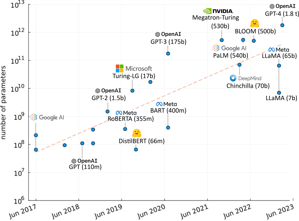
In 2018 OpenAI released a paper titled Improving Language Understanding by Generative Pre-Training. This led to the development of their first Generative Pre-trained Transformer (GPT) model. As of 2024 they have released four versions of GPT, with the latest requiring over 1.8 trillion parameters. The interactive version of the model, ChatGPT, has gained widespread fame for its human like responses.
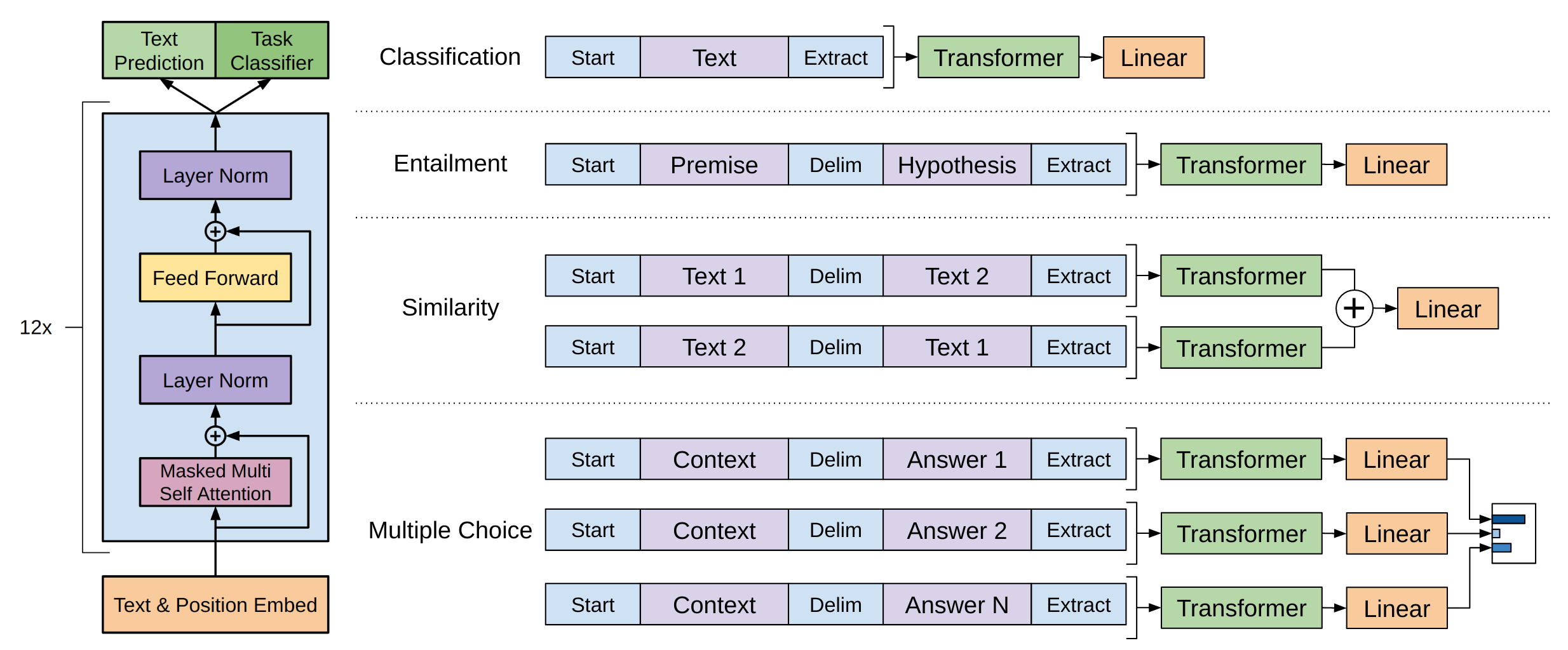
The goal of this post is to create a generative transformer following OpenAI’s methodology for their first GPT-1 paper. It will be a vanilla transformer without many of the additions that have been proposed in this fast paced field. The model will be trained on Shakespeare plays and will be able to generate text that looks and sounds like Shakespeare. This model can then be used as the pre-trained foundation for further supervised tasks.
Outcome
The goal is to create a model which implements the architecture in the GPT paper:
TransformerGenerator(
  Embedding(72 => 32),                  # 2_304 parameters
  Embedding(64 => 32),                  # 2_048 parameters
  Dropout(0.1),
  TransformerBlock(
    MultiHeadAttention(
      nhead=4,
      denseQ = Dense(32 => 32; bias=false),  # 1_024 parameters
      denseK = Dense(32 => 32; bias=false),  # 1_024 parameters
      denseV = Dense(32 => 32; bias=false),  # 1_024 parameters
      denseO = Dense(32 => 32),         # 1_056 parameters
    ),
    LayerNorm(32),                      # 64 parameters
    Dense(32 => 128, relu),             # 4_224 parameters
    Dense(128 => 32),                   # 4_128 parameters
    LayerNorm(32),                      # 64 parameters
    Dropout(0.1),
  ),
  ..., # 2x more TransformerBlocks
  Dense(32 => 72),                      # 2_376 parameters
  mask = 64×64 Matrix{Bool},
)        # Total: 43 trainable arrays, 44_552 parameters,
          # plus 1 non-trainable, 4_096 parameters, summarysize 180.641 KiB.
It will map tokens to indices and will operate on those :
mask = make_causal_mask(ones(8, 8))
indices = indexer(collect("LYSANDER")) # [23, 36, 30, 12, 25, 15, 16, 29]
model(indices; mask=mask)
It will return a $ V \times n $ matrix, where $V$ is the vocabulary size and $n$ is the length of the input vector (8 in this example). Each column represents logits for each token. These will then be normalised to values between 0 and 1 using the softmax function. The model will be trained so that each value represents the probability of the next most likely token based on all the tokens before, up to a fixed context length $n$. As a whole the matrix represents the probabilities associated with shifting the input one value to the right.
As an example, during training the input will be “LYSANDER” and the reference “YSANDER\n”. The model will output a probability matrix and after sampling the result will be something like “YSANDR\nH”. This is then compared to the reference to improve the output.
The model computes all the probabilities for all $n$ characters in parallel through the same set of matrix operations, which makes this very efficient during training. We will effectively compare $n$ different predictions for one sample. However at inference time we are only interested in the last ($n$th) character, because we already have the first $n$ characters. Therefore we will discard the first $n-1$ predictions. (They would have already been used internally in the model.)
This is an inherent inefficiency in the transformer model architecture. (KV Caching can be used to overcome it. See João Lages’ visual explanation or a later blog post.)
Generation will repeat inference many times, each time adding the last generated token to the context and generating a new token. The result is something like:
CLATIO.
No, Goe, him buchieds is, hand I was,
To queer thee that of till moxselat by twish are.

BENET.
Are warrain Astier, the Cowlles,
bourse and nope, Merfore myen our to of them coun-mothared man,
Here is
Mafter my thath and herop, and in in have low’t so, veriege a the can eeset thy
inscestle marriom.

ADY.
Thus him stome
To so an streeward. Here cas, which id renuderser what thou bee of as the hightseleh-to.

CHAESS.
With he mand, th’ fouthos. I purcot Lay,
You.

GATHENT.
Who, to hath fres
This was generated by a tiny 42,400 parameter model with a perplexity of 6.3, down from a random sampling perplexity of 71 for 71 characters.
Background
In May 2022 I wrote a blog post on transformers from first principles in Julia. It developed a transformer for a classification task, namely predicting stars for Amazon Reviews. That post was lacking however in that it did not create a decoder transformer. This post is dedicated to that task. I’ve written this as a stand-alone from the original even though much of the code is the same. I refer back to the original post for some explanations. Please see the Design Considerations section which is not repeated here.
This post was inspired by Andrej Karpathy’s Zero to Hero course. I highly recommend it. It covers many ideas like backpropagation, normalisation and embeddings that are assumed knowledge in this post. In particular, this post emulates lesson 7 except the language and framework used are Julia and Flux.jl, not Python and PyTorch. The source code can be accessed at Karpathy’s famed nanoGPT repository.
My own repositories with the code in this blog post can be accessed at TransformersLite.jl and TransformersLite-examples. I will not detail any “pretty” printing function here - please see the repository for those.
This is not meant to be a full scale Julia solution. For that, please see the Transformers.jl package. It has better optimizations, APIs for HuggingFace and more.
2 Data
2.1 Download
The Complete Works of William Shakespeare by William Shakespeare has no copyright attached and can be downloaded legally from Project Gutenburg.
Here is a line to download it with cURL:
curl https://www.gutenberg.org/cache/epub/100/pg100.txt > project_gutenberg_shakespeare.txt
2.2 Preparation
A typical passage from the text looks like:
LYSANDER.
How now, my love? Why is your cheek so pale?
How chance the roses there do fade so fast?

HERMIA.
Belike for want of rain, which I could well
Beteem them from the tempest of my eyes.

LYSANDER.
Ay me! For aught that I could ever read,
Could ever hear by tale or history,
The course of true love never did run smooth.
But either it was different in blood—
This is what we want the transformer to learn and the vast majority of the text follows this format. However some pieces do not. These include the Project Gutenberg introduction and conclusion, the table of contents, the sonnets, the preambles - these list the acts and scenes in each play - and so on. Those should all be removed.
Optionally, the small amount of non-ASCII characters (œ, Æ,æ, …) should be removed. I also removed the “&” symbol and changed the archaic usage of “&c.” to “etc.”.
I’ve made a script which does all this work, prepare_shakespeare.jl. It reduces the file size from 5.4 MB to 4.8 MB.
2.3 Exploration
We can load the text in Julia with:
text = open(filepath) do file
    read(file, String)
end
Some basic statistics:
count('\n', text)   # 182,027 lines
count("\n\n", text) # 38,409 passages
count(r"\w+", text) # 921,816 words
length(text)        # 4,963,197 characters
The prepared dataset contains 182,027 lines spanning over approximately 38,409 passages, 921,816 words and 4,963,197 characters.
Most passages are very short - less than 100 characters. The longest is Richard’s monologue in “The Third Part of King Henry the Sixth” which consists of 3047 characters.
Lines have an average of 26.27 characters with the longest being 77 characters in length.
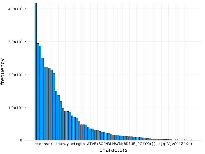
After the data preparation there are 71 unique characters in the text: \n !(),-.:;?ABCDEFGHIJKLMNOPQRSTUVWXYZ[]_abcdefghijklmnopqrstuvwxyz—‘’“”
There are approximately 30,040 unique words in the dataset. Of these, approximately 80% appear less than 10 times and 96.5% less than 100 times. The most frequent word is “the” with 23,467 occurrences.
3 Model
3.1 Project Setup
To start, make a package in the Julia REPL:
cd("path\\to\\project")
] # enter package mode
generate TransformersLite # make a directory structure
dev "path\\to\\project\\TransformersLite"
The purpose of making a package is that we can now use the super helpful Revise package, which will dynamically update most changes during development without errors:
julia> using Revise
julia> using TransformersLite
The following packages need to be loaded/added for this tutorial:
julia> using Flux, LinearAlgebra, NNlib, ProgressMeter, Random, StatsBase3.2 Tokenization
The model will predict probabilities for each token in a given vocabulary. There is a choice as to what constitutes a token. One extreme is one token for each word in the dataset. Here there are far too many unique words so it will explode the parameter count while providing too few training samples per token. The other extreme is character level tokens. This compresses the learning space too much to get fully realistic outputs, but otherwise it works surprisingly well. In between is sub-word tokenization such as Byte Pair Pair encoding. This allows configurable vocabulary lengths. See my TokenizersLite.jl package, the BytePairEncoding.jl package or Karpathy’s latest video.
Here we will follow Karpathy’s approach and use character level tokens. The model will learn to predict each word character by character.
First get all the characters:
characters = sort(collect(Set(text)))Karpathy uses two dictionaries to convert between characters and indices: char_to_int and int_to_char.
I’m going to wrap these in a slightly more complex IndexTokenizer struct introduced in my first post.
It holds a vector of the vocabulary (equivalent to int_to_char) and a lookup for reversing this (equivalent to char_to_int).
Additionally, it has an unknown symbol if any of the characters are not in the vocabulary.
The constructor is as follows:
struct IndexTokenizer{T}
    vocabulary::Vector{T}
    lookup::Dict{T, Int}
    unksym::T
    unkidx::Int
    function IndexTokenizer(vocab::Vector{T}, unksym::T) where T
        if !(unksym ∈ vocab)
            pushfirst!(vocab, unksym)
            unkidx = 1
        else
            unkidx = findfirst(isequal(unksym), vocab)
        end
        lookup = Dict(x => idx for (idx, x) in enumerate(vocab))
        new{T}(vocab, lookup, unksym, unkidx)
    end
end

Base.length(tokenizer::IndexTokenizer) = length(tokenizer.vocabulary)

function Base.show(io::IO, tokenizer::IndexTokenizer)
    T = eltype(tokenizer.vocabulary)
    print(io, "IndexTokenizer{$(T)}(length(vocabulary)=$(length(tokenizer)), unksym=$(tokenizer.unksym))")
end
For encoding we lookup the character in the dictionary, returning the index of the unknown symbol by default:
function encode(tokenizer::IndexTokenizer{T}, x::T) where T
    get(tokenizer.lookup, x, tokenizer.unkidx)
end

function encode(tokenizer::IndexTokenizer{T}, seq::AbstractVector{T}) where T
    map(x->encode(tokenizer, x), seq)
end
We can add a method to do multiple dispatch on the type IndexTokenizer itself
which turns the struct into a function:
(tokenizer::IndexTokenizer)(x) = encode(tokenizer, x)Encoding example:
push!(characters, 'Ø') # unknown symbol
vocab_size = length(characters) # 72
indexer = IndexTokenizer(characters, 'Ø')
tokens = indexer(collect("How now, my love?")) # [19, 55, 63, 2, 54, ..., 62, 45, 11]
Decoding goes the other way:
decode(tokenizer::IndexTokenizer{T}, x::Int) where T =
	0 <= x <= length(tokenizer) ? tokenizer.vocabulary[x] : tokenizer.unksym

function decode(tokenizer::IndexTokenizer{T}, seq::Vector{Int}) where T
    map(x->decode(tokenizer, x), seq)
end
An example:
join(decode(indexer, [23, 36, 30, 12, 25, 15, 16, 29])) # LYSANDER3.3 Embeddings
Each token is transformed into a vector of floating point numbers. This vector represents some sort of meaning in a large, abstract vector space, where vectors that are closer to each other are more similar. (There is plenty of literature on this subject.)
Flux.jl comes with an embedding layer which can be used directly:
embedding = Flux.Embedding(72 => 32)
x = rand(1:72, 10) # [40, 49, 55, 65, 27, 50, 35, 69, 40, 29]
embedding(x) # 32×10 Matrix{Float32}
Here is the source code:
struct Embedding{W<:AbstractMatrix}
  weight::W
end

Flux.@layer Embedding

Embedding((in, out)::Pair{<:Integer, <:Integer}; init = randn32) = Embedding(init(out, in))

(m::Embedding)(x::Integer) = m.weight[:, x]
(m::Embedding)(x::AbstractVector) = NNlib.gather(m.weight, x)
(m::Embedding)(x::AbstractArray) = reshape(m(vec(x)), :, size(x)...)

function Base.show(io::IO, m::Embedding)
  print(io, "Embedding(", size(m.weight, 2), " => ", size(m.weight, 1), ")")
end
This struct stores a weight, by default the smaller datatype of Float32 rather than the usual Julia default of Float64.
This saves on space without reducing accuracy.
(Float16, Float8 and as low as Float4 are all used in machine learning models.)
On the forward pass each index is used to retrieve the associated column vector from the matrix.
However instead of using m.weight[:, x] the function uses NNlib.gather(m.weight, x).
This is because gather comes with an rrule defined for it (source):
∇gather_src(Δ, src_size, idx) = scatter!(+, fill!(similar(Δ, eltype(Δ), src_size), 0), Δ, idx)The rrule is a reverse (backwards) rule that encodes the derivative for backpropagation.
It is what makes the magic of automatic differentiation work.
The function gather does not have a formal derivative, but scatter is the opposite of it and is what we need to apply when we calculate the loss:
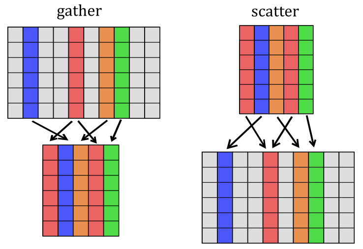
At the end of backpropagation we need to distribute the error matrix amongst the original word embeddings.
This is what scatter does. Note that we use the red column twice, so we have two error columns directed towards it.
The rrule applies + as the reducing function; that is, the two errors are added together and then to the word embedding.
Scatter can be inefficient. If we do a small experiment and call scatter we will see it results in a large matrix of mostly zeros:
NNlib.scatter(+, rand(8, 4), [1, 5, 11, 1]; dstsize=(8, 15))
8×15 Matrix{Float64}:
 1.62703   0.0  0.0  0.0  0.495725  0.0  0.0  0.0  0.0  0.0  0.237452     0.0  0.0  0.0  0.0
 0.979735  0.0  0.0  0.0  0.984499  0.0  0.0  0.0  0.0  0.0  0.145738     0.0  0.0  0.0  0.0
 0.892948  0.0  0.0  0.0  0.76959   0.0  0.0  0.0  0.0  0.0  0.714658     0.0  0.0  0.0  0.0
 1.45113   0.0  0.0  0.0  0.883492  0.0  0.0  0.0  0.0  0.0  0.52775      0.0  0.0  0.0  0.0
 0.702824  0.0  0.0  0.0  0.965256  0.0  0.0  0.0  0.0  0.0  0.0966964    0.0  0.0  0.0  0.0
 1.16978   0.0  0.0  0.0  0.568429  0.0  0.0  0.0  0.0  0.0  0.000161501  0.0  0.0  0.0  0.0
 1.80566   0.0  0.0  0.0  0.271676  0.0  0.0  0.0  0.0  0.0  0.430018     0.0  0.0  0.0  0.0
 1.16445   0.0  0.0  0.0  0.911601  0.0  0.0  0.0  0.0  0.0  0.786343     0.0  0.0  0.0  0.0
3.4 Position encoding
The matrix operations used in the transformer are parallel operations. This speeds up computation and is a major reason why they are so popular. However this is an issue: they do not take order into account. We can shuffle the columns in the embedding matrix and it will not affect the output.

To counter-act this, the authors of the Attention is all you need (2017) paper suggested adding a second embedding to the first where the indices are the positions in the sequence.1
We can use an Embedding matrix as before, except with a different input:
position_encoding = Embedding(16 => 32)
x = rand(32, 10) # the output of the first embedding layer
indices = 1:size(x, 2) # 1:10
embedding(indices) # 32×10 Matrix{Float32}
Other position encodings
Transformers are an active area of research and many position encodings have been proposed.
- Sinusodial Position Encodings: The original paper gave equations to calculate a fixed embedding matrix. For an explanation and implementation see my first post.
- Relative Position Embeddings (RPE) (2018): add embeddings in the attention step where each entry relates $r=j_k-i_q$. The Music Transformer (2018) paper greatly improved computation of this matrix. For a helpful video see Relative Self-Attention Explained.
- Rotary Position Embeddings (RoPE) (2023): encode absolute position with a fixed rotation matrix, which handles longer sequences better and encodes relative positions better than sinusoidal embeddings. A downside is every
keyandqueryin the attention step needs to be multiplied by this rotation matrix instead of adding an encoding once at the start. - Position Interpolation (2023): extending embedding matrices by linearly down-scaling the input position indices to match the original context window size. For example, each index in a 128 context window can be down-scaled by a factor of 2 to match a 64 length encoding matrix. Half indices like 42.5 are a linear combination of the indices before and after (so 42 and 43). Some fine tuning is required for best results. This can be combined with RoPE.
This embedding matrix restricts the context size. In the example the embedding matrix is 32×16 so a maximum of 16 tokens that can be passed to the model at time. To overcome this a sliding window must be implemented and the model will completely “forget” any character outside of the window.
Ideally we would create an embedding matrix as large as possible so that the bottleneck is the training data, not the model. However attention, which will be discussed in the next section, scales with $n^2$ for a context length $n$. This is a significant performance penalty for a larger context size.
3.5 Attention
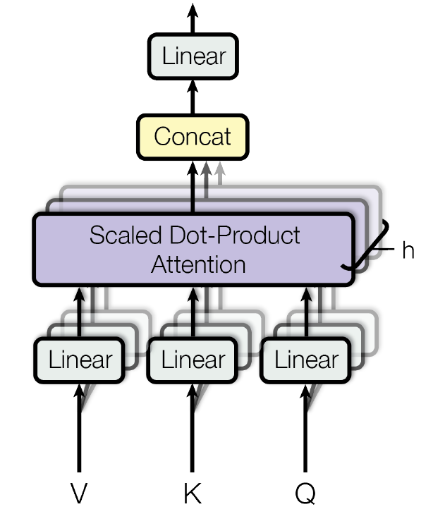
- Definition
- Masking
- Batched multiplication
- MultiHeadAttention layer
- Multi-Head Attention
- Scaled Dot Attention
- Full example
3.5.1 Definition
Attention is the main mechanism at the heart of the transformer. Theoretically it is a weighting of every token towards every other token, including itself. It is asymmetrical and so forms a full $n \times n$ matrix. For example consider word level tokens for the sentence “The elephant in the room”. The tokens “The”, “in”, “the” and “room” might all rate “elephant” the highest, but “elephant” will probably only rate “room” highly.
The attention equation is: \(A = V\text{softmax}\left(\frac{1}{\sqrt{d_h}}K^T Q\right) \label{eq:attention} \tag{3.6.1}\)
where $\text{softmax}$ is given by:
\[\text{softmax}(z, i) = \frac{e^{z_i}}{\sum_r^V e^{z_r}} \label{eq:softmax} \tag{3.6.2}\]Its calculation scales with $\mathcal{O}(n^2d_h)$ where $n$ is the input token length and $d_h$ is the head dimension, also known as the hidden dimension.
Efficient self-attention
Given the $n^2$ scaling of attention much effort has gone into altering this step. This includes sparse attention layers, factorisation/kernels for linear attention and down-sampling. A detailed survey can be found at Efficient Transformers: A Survey (2020). All these alternatives are faster than attention but come at the expense of accuracy.
Another line of research is to improve the computation. This include Flash attention (2022) which improves computational efficiency on a single GPU while Ring attention (2023) aims to distribute the work efficiently across multiple devices.
Here the key $K$, query $Q$ and value $V$ are derived from the input matrix $X$ using weights:
\[\begin{align} K = W_K X \\ Q = W_Q X \\ V = W_V X \end{align}\]Each weight $W$ has a size $d_h \times d_\text{emb}$ and the input matrix has a size $d_\text{emb} \times n$ where $d_\text{emb}$ is the embedding dimension. Each of these matrices therefore has a size $d_h \times n$.
From this we can show that the first matrix product is a weighted dot product of every vector to every other vector in the input matrix, resulting in a $n \times n$ matrix:
\[K^T Q = (W_KX)^T(W_QX) = X^T W_K^T W_Q X\]This is then following by scaling ($1/\sqrt{d_h}$) and normalisation ($\text{softmax}$). Lastly this matrix is used as a weight for $V$. The output is $d_h \times n$.
3.5.2 Masking
There is a flaw in this architecture. The attention is computed across all tokens at once. This means that past tokens will be given access to future tokens. However the training objective is to predict future tokens. Therefore only the $n$th token, whose next token is missing, will be trained fairly.
To overcome this the authors of the Attention (2017) paper suggested masking the matrix before the softmax with $-\infty$ at each illegal connection, so that $\exp(-\infty)=0$ which effectively removes their influence.
The masked matrix will look like:
\[\begin{bmatrix} s_{11} & s_{12} & s_{13} &... & s_{1n} \\ -\infty & s_{22} & s_{23} &... & s_{2n} \\ -\infty & -\infty & s_{33} &... & s_{3n} \\ \vdots & \vdots & \vdots & \ddots & \vdots \\ -\infty & -\infty & -\infty & ... & s_{nn} \end{bmatrix}\]Firstly a mask is made where all valid connections have a true and all illegal connections have a false.
Here is the code from NNlib.jl:
using LinearAlgebra
function make_causal_mask(x::AbstractArray; dims::Int=2)
  len = size(x, dims)
  mask = triu(trues_like(x, (len, len)))
  mask
end

trues_like(x::AbstractArray, sz=size(x)) = fill!(similar(x, Bool, sz), true)
Dataless masks
We don't have to allocate memory to create a mask. The causal mask is defined by $j \geq i$ for all indices $i$, $j$. We can write this as a function as long as we can also write an equivalent rrule for it as well. See NeuralAttentionlib.jl for such an implementation.
The mask will be applied through ifelse, where trues maintain their value but the falses are replaced with some large negative number.
apply_mask(logits, mask::Nothing) = logits

function apply_mask(logits, mask)
    neginf = typemin(eltype(logits))
    ifelse.(mask, logits, neginf)
end
Usage:
mask = make_causal_mask(ones(5, 5))
x = randn(Float32, 5, 5)
apply_mask(x, mask) # 5×5 Matrix{Float32}:
Backpropagation:
using Flux: pullback
y, back = pullback(apply_mask, x, mask);
grads = back(randn(size(y)...))
grads[1] # zero where -inf
As an experiment, set the mask to nothing during training.
It should be possible to get very low training losses (below 0.5) corresponding to very low perplexities (less than 2) with very small models but without a corresponding increase in generation quality.
3.5.3 Batched multiplication
The Attention (2017) paper suggested a further enhancement on attention where the input matrix is divided amongst $H$ heads. This results in a $\tfrac{d_\text{emb}}{H} \times n \times H$ array. Furthermore, working with batches adds an extra dimension: $d_h \times n \times H \times B$.
We could work with these arrays as Vector{<:Matrix{T}} and Vector{<:Vector{<:Matrix{T}}} respectively, but it is more efficient to work with them as Array{T, 3} and Array{T, 4} because then we can work with optimised array functions.
My first post goes into more detail about multiplication with higher order arrays.2 It compares vanilla versions with optimised versions. Here I will present the optimised version only.
Batch multiplication is defined as:
\[C_{ijk} = \sum_r A_{irk} B_{rjk}\]An optimised version is available through the NNlib.jl library, a dependency of Flux.jl:
using NNlib
A = rand(6, 8, 4);
B = rand(8, 5, 4);
NNlib.batched_mul(A, B) # 6×5×4 Array{Float64, 3}
The 4D batched multiplication is defined as:
\[C_{ijkl} = \sum_r A_{irkl} B_{rjkl}\]We can calculate this array with the same batched_mul by reshaping any 4D $m\times n \times p \times q$ arrays into 3D $m\times n \times pq$ arrays, do the multiplication, and reshape back.
This is exactly what the implementation does behind the scenes:
using NNlib
A = rand(6, 8, 4, 3);
B = rand(8, 5, 4, 3);
NNlib.batched_mul(A, B) # 6×5×4×3 Array{Float64, 4}
The Flux Dense layer does something similar.
3.5.4 MultiHeadAttention layer
Flux.jl now comes with a Flux.MultiHeadAttention layer.
However for continuity with my first post, I will present my own MultiheadAttention layer except now with masking.
It is very similar to the code in Flux.jl and NNlib.jl.
The differences are in design choices for the inputs and Flux.jl’s implementations are slightly more generic.
First define a struct to hold all the dense layers and a parameter for $H$ called nhead:
struct MultiheadAttention{Q<:Dense, K<:Dense, V<:Dense, O<:Dense}
    nhead::Int
    denseQ::Q
    denseK::K
    denseV::V
    denseO::O
end

#= tell Flux which parameters are trainable =#
Flux.@layer MultiHeadAttention trainable=(denseQ, denseK, denseV, denseO)
The model is defined by 4 values: the number of heads $H$, the input dimension $d_\text{in}$, the output dimension $d_\text{out}$ and the head dimension $d_h$. The default for $d_h$ is $d_\text{in}/H$.
function MultiheadAttention(
    nhead::Int, dim_in::Int, dim_head::Int, dim_out::Int
    )
    MultiheadAttention(
        nhead,
        Dense(dim_in, dim_head*nhead; bias=false),
        Dense(dim_in, dim_head*nhead; bias=false),
        Dense(dim_in, dim_head*nhead; bias=false),
        Dense(dim_head*nhead, dim_out),
    )
end

function MultiheadAttention(
    nhead::Int, dim_in::Int, dim_out::Int
    )
    if dim_in % nhead != 0
        error("input dimension=$dim_in is not divisible by number of heads=$nhead")
    end
    MultiheadAttention(nhead, dim_in, div(dim_in, nhead), dim_out)
end
Now for the forward pass.
In general there are three input matrices with the names of key, query and value.
Later we will pass the same value x for all of them.
From these we can calculate $Q$, $K$ and $V$ and pass them to the multi_head_scaled_dot_attention function:
function (mha::MultiheadAttention)(query::A3, key::A3, value::A3
    ; kwargs...) where {T, A3 <: AbstractArray{T, 3}}
    Q = mha.denseQ(query)
    K = mha.denseK(key)
    V = mha.denseV(value)
    A, scores = multi_head_scaled_dot_attention(mha.nhead, Q, K, V; kwargs...)
    mha.denseO(A), scores
end
This layer returns the scores as well, like Flux.jl’s MultiheadAttention layer.
These are useful for inspecting the model.
3.5.5 Multi-Head Attention
The multi_head_scaled_dot_attention begins as follows:
function multi_head_scaled_dot_attention(nhead::Int, Q::A3, K::A3, V::A3
    ; kwargs...) where {T, A3 <: AbstractArray{T, 3}}
    qs = size(Q)
    ks = size(K)
    vs = size(V)
    dm = size(Q, 1)
    dh = div(dm, nhead)
The $Q$, $K$ and $V$ matrices need to be split from $d_m \times N \times B$ to $d_h \times N \times H \times B$. This is done in two steps:
- $(d_h \times H)\times N \times B$ (break $d_m$ into $d_h$ and $H$)
- $d_h \times N \times H \times B$ (swap the 2nd and 3rd dimensions)
    Q = permutedims(reshape(Q, dh, nhead, qs[2], qs[3]), [1, 3, 2, 4])
    K = permutedims(reshape(K, dh, nhead, ks[2], ks[3]), [1, 3, 2, 4])
    V = permutedims(reshape(V, dh, nhead, vs[2], vs[3]), [1, 3, 2, 4])
Then we calculate the scaled dot attention for each head, combine results and return it:
    A, scores = scaled_dot_attention(Q, K, V; kwargs...)
    A = permutedims(A, [1, 3, 2, 4])
    A = reshape(A, dm, size(A, 3), size(A, 4))
    A, scores
end
3.5.6 Scaled Dot Attention
The scaled dot attention is defined by default for 3D arrays. $Q$ is of size $d_h \times d_q \times H$ while $K$ and $V$ are both of size $d_h \times d_{kv} \times H$. Usually $n=d_q=d_{kv}$.
function scaled_dot_attention(
    query::A3, key::A3, value::A3
    ; mask::Union{Nothing, M}=nothing
    ) where {T, A3 <: AbstractArray{T, 3}, M <: AbstractArray{Bool}}
    dh = size(query, 1)
    keyT = permutedims(key, (2, 1, 3)) # (dkv, dh, nhead)
    atten = one(T)/convert(T, sqrt(dh)) .* batched_mul(keyT, query) # (dkv, dh, nhead)*(dh, dq, nhead) => (dkv, dq, nhead)
    atten = apply_mask(atten, mask) # (dkv, dq, nhead)
    scores = softmax(atten; dims=1) # (dkv, dq, nhead)
    batched_mul(value, scores), scores # (dh, dkv, nhead)*(dkv, dq, nhead) => (dh, dq, nhead)
end
As explained above, we need to reshape 4D arrays into 3D arrays, apply the usual scaled dot attention and then reshape back:
function scaled_dot_attention(query::A4, key::A4, value::A4
    ; kwargs...) where {T, A4 <: AbstractArray{T, 4}}
    batch_size = size(query)[3:end]
    Q, K, V = map(x -> reshape(x, size(x, 1), size(x, 2), :), (query, key, value))
    A, scores = scaled_dot_attention(Q, K, V; kwargs...)
    A = reshape(A, (size(A, 1), size(A, 2), batch_size...))
    scores = reshape(scores, (size(scores, 1), size(scores, 2), batch_size...))
    A, scores
end
3.5.7 Full example
Model:
mha = MultiheadAttention(4, 32, 32)
Flux._big_show(stdout, mha)
#=
MultiheadAttention(
  4,
  Dense(32 => 32; bias=false),          # 1_024 parameters
  Dense(32 => 32; bias=false),          # 1_024 parameters
  Dense(32 => 32; bias=false),          # 1_024 parameters
  Dense(32 => 32),                      # 1_056 parameters
)                   # Total: 5 arrays, 4_128 parameters, 16.422 KiB.
=#
Forward pass:
x = randn(Float32, 32, 20, 2) # d×n×B
mask = make_causal_mask(ones(32, 20))
y, scores = mha(x, x, x; mask=mask) # 32×20×2 Array{Float32, 3}, 20×20×4×2 Array{Float32, 4}
Backpropagation:
using Flux
loss = sum # dummy loss function
grads = Flux.gradient(m -> loss(m(x, x, x; mask=mask)[1]), mha)
keys(grads[1]) # (:nhead, :denseQ, :denseK, :denseV, :denseO)
3.6 Transformer Blocks
The other components we need for the transformer block are Layer Norm, Feed Forward (two consecutive dense layers) and dropout. We can use the Flux.jl implementations for these.
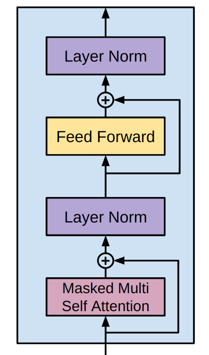
This means we can now create a transformer block:
struct TransformerBlock{
    MHA<:MultiheadAttention,
    N1<:LayerNorm,
    D1<:Dense,
    D2<:Dense,
    N2<:LayerNorm,
    DO<:Dropout}
    multihead_attention::MHA
    norm_attention::N1
    dense1::D1
    dense2::D2
    norm_feedforward::N2
    dropout::DO
end

Flux.@layer TransformerBlock # make whole layer trainable
This whole block can be defined with only 5 parameters:
- The number of heads $H$.
- The dimension $d$.
- The hidden dimension for the feed-forward network. The convention is $4d$.
- The activation function.
- A drop out probability.
In code:
TransformerBlock(
    nhead::Int,
    dim_model::Int,
    dim_hidden::Int;
    act=relu,
    pdrop::Float64=0.1,
    ) = TransformerBlock(
    MultiheadAttention(nhead, dim_model, dim_model),
    LayerNorm(dim_model),
    Dense(dim_model, dim_hidden, act),
    Dense(dim_hidden, dim_model),
    LayerNorm(dim_model),
    Dropout(pdrop),
)
There are skip connections in the forward pass:3
function (t::TransformerBlock)(x::A; mask::M=nothing) where {
    A<:AbstractArray, M<:Union{Nothing, AbstractArray{Bool}}}
    h, scores = t.multihead_attention(x, x, x; mask=mask) # (dm, N, B)
    h = t.dropout(h)
    h = x + h
    h = t.norm_attention(h)     # (dm, N, B)
    hff = t.dense1(h)           # (dh, N, B)
    hff = t.dense2(hff)         # (dm, N, B)
    hff = t.dropout(hff)
    h = h + hff
    h = t.norm_feedforward(h)   # (dm, N, B)
    h
end
Model:
block = TransformerBlock(4, 32, 32*4)
Flux._big_show(stdout, block)
#=
TransformerBlock(
  ...
)  # Total: 13 arrays, 12_608 parameters, 50.234 KiB.
=#
Forward pass:
x = randn(Float32, 32, 20, 2) # d×n×B
mask = make_causal_mask(ones(32, 20)) # 20×20 Matrix{Bool}
y = block(x; mask=mask) # 32×20×2 Array{Float32, 3}
Backpropagation:
loss = sum # dummy loss function
grads = Flux.gradient(m -> loss(m(x; mask=mask)), block)
keys(grads[1]) # (:multihead_attention, :norm_attention, :dense1, :dense2, :norm_feedforward, :dropout)
3.7 Generator
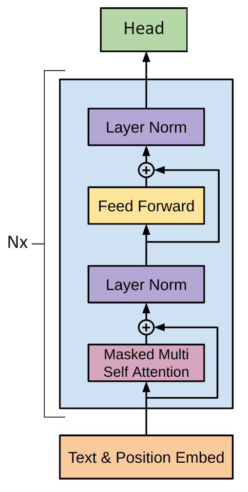
We will create a struct to hold the generator.
struct TransformerGenerator{
    E<:Flux.Embedding,
    PE<:Flux.Embedding,
    DO<:Dropout,
    TB<:Vector{<:TransformerBlock},
    D<:Dense,
    M<:Union{Nothing, AbstractMatrix{Bool}},
    }
    embedding::E
    position_encoding::PE
    dropout::DO
    blocks::TB
    head::D
    mask::M # optional buffer
end

Flux.@layer TransformerGenerator trainable=(embedding, position_encoding, blocks, dropout, head)
By default the forward pass will use the model’s mask, else the user can pass a mask to it:
function (t::TransformerGenerator)(x::A; mask::M=t.mask) where {
    A<:AbstractArray, M<:Union{Nothing, AbstractMatrix{Bool}}}
    x = t.embedding(x)              # (dm, N, B)
    N = size(x, 2)
    x = x .+ t.position_encoding(1:N) # (dm, N, B)
    x = t.dropout(x)                # (dm, N, B)
    for block in t.blocks
        x = block(x; mask=mask)     # (dm, N, B)
    end
    x = t.head(x)                   # (vocab_size, N, B)
    x
end
Create a model:
context_size = 64
dim = 32
nheads = 4
vocab_size = 71
mask = make_causal_mask(ones(context_size, context_size))
model = TransformerGenerator(
    Embedding(vocab_size => dim),
    Embedding(context_size => dim),
    Dropout(0.1),
    TransformerBlock[
        TransformerBlock(4, dim, dim * 4; pdrop=0.1),
        TransformerBlock(4, dim, dim * 4; pdrop=0.1),
        TransformerBlock(4, dim, dim * 4; pdrop=0.1),
    ],
    Dense(dim, vocab_size),
    copy(mask)
)
Flux._big_show(stdout, model)
#=
TransformerGenerator(
  ...
)         # Total: 43 trainable arrays, 44_487 parameters,
          # plus 1 non-trainable, 4_096 parameters, summarysize 180.410 KiB.
=#
We can test it with a random vector of indices:
x = reshape(rand(1:vocab_size, 34), :, 1) # make it a batch of 1
mask = make_causal_mask(ones(dim, length(x)))
y = model(x; mask=mask) # 71×34×1 Array{Float32, 3}
Or a random batch:
X = rand(1:vocab_size, 34, 10)
Y = model(X; mask=mask) # 71×34×10
3.8 Generation
Let’s now generate text with the model.
The model has a fixed context length. To generate text longer than this fixed length we will implement a sliding window. This window will take the last $n$ tokens (rows) of the current context for each column (sample) in the batch:
function tail(A::AbstractMatrix, n::Int)
    n = min(n, size(A, 1))
    A[(end - n + 1):end, :]
end
The transformer generates a $V\times N \times B$ matrix. We will only take the logits for the last token per iteration, resulting in a $V\times B$ matrix. These logits will be converted to probabilities via the softmax function $\ref{eq:softmax}$.
We have a choice of how to sample these probabilities. The greedy approach is to always take the token with the maximum probability. A better approach is to randomly sample based on the probabilities. That way a token with a high probability is more likely to be chosen, but it is not guaranteed. This gives us some diversity in the results. We then add this to the context and repeat.
The full function is:
using Random, StatsBase
function generate(
    rng::AbstractRNG, model::TransformerGenerator, context::AbstractMatrix{T}
    ; context_size::Int, max_tokens::Int=100,
    ) where T
    for i in 1:max_tokens
        context_crop = tail(context, context_size)
        n = size(context_crop, 1)
        mask = isnothing(model.mask) ? nothing : view(model.mask, 1:n, 1:n)
        logits = model(context_crop; mask=mask) |> cpu # (vocab_size, n, B)
        logits = logits[:, end, :] # (vocab_size, B)
        context_next = multinomial_sampling(rng, logits)
        context = cat(context, context_next; dims=1)
    end
    context
end

function generate(model::TransformerGenerator, context::AbstractMatrix; kwargs...)
    generate(Random.default_rng(), model, context; kwargs...)
end

function multinomial_sampling(rng::AbstractRNG, logits::AbstractMatrix)
    probs = softmax(logits; dims=1)
    tokens = [sample(rng, Weights(p)) for p in eachcol(probs)]
    tokens
end
Testing it out:
context = reshape([1], 1, 1) # start with the new line symbol
out = generate(model, context; context_size=64) # 101×1 Matrix{Int64}
Decode the output using the tokenizer from section 3.2:
decoded_text = join(decode(indexer, out[:, 1]))
print(decoded_text)
The output:
A[RH N)pEy.QEgs?YbgnRsz-ZRDdUXvU Pzwzzxukvv_P;goxe(G;C;I
RIgB ‘E[xIqZ-J;gK—wwEUTZYtUg:tEhl-kZ;s:x.ggt
This is nonsense. The model does no better than drawing each character randomly. We need to train the model to get something sensible out of it.
4 Training
4.1 Train/validation split
It is always good practice to split the data into train, validation and test splits. For simplicity, we’ll only use a train and validation split. We’ll put the first 95% of data in the train split and the remainder in the validation split.4
tokens = indexer(collect(text))
n_val = floor(Int, (0.95) * length(tokens))
train_data = tokens[1:n_val]
val_data = tokens[(n_val + 1):end]
4.2 Batch generation
The model will be trained on segments of the text which match the context length $n$. For a text of length $L$ there are $L-n+1$ characters we can select to be the first character of the segments, excluding the last $n-1$ characters. For the Shakespeare text, this results in approximately 4.9 million different segments.
There is however plenty of overlap so we don’t have to train on all of them. We can instead randomly sample segments from the text. Characters at any point in the text will have a probability of appearing of $p\approx n/L$ (the ends are less likely). For many steps $s$ this binomial distribution can be approximated with a normal distribution with a mean $sp\approx sn/L$ and standard deviation $\sqrt{sp(1-p)}\approx \sqrt{sn/L}$. For example, for 4.9 million characters, a context length of 64 and 100,000 steps, each character at each point will appear 1.31±1.14 times.
The other important task is to create the reference text that the model will be trained to generate, which is simply the input text shifted by one. (This reduces the number of valid segments by 1.)
The function is as follows:
using Random
function get_shifted_batch(rng::AbstractRNG, data::AbstractVector, context_size::Int, batch_size::Int)
    indices = rand(rng, 1:(length(data)-context_size), batch_size)
    X = similar(data, context_size, batch_size)
    Y = similar(data, context_size, batch_size)
    for (j, idx) in enumerate(indices)
        X[:, j] = data[idx:(idx + context_size - 1)]
        Y[:, j] = data[(idx + 1):(idx + context_size)]
    end
    X, Y
end

get_shifted_batch(data::AbstractVector, context_size::Int, batch_size::Int) =
    get_shifted_batch(Random.default_rng(), data, context_size, batch_size)
Usage:
text = rand(1:72, 1000) # pretend we've already indexed it
rng = MersenneTwister(2)
X, Y = get_shifted_batch(rng, text, 4, 3)
The outputs look like:
    X              Y
 1   70  66  |   9  60   3
 9   60   3  |  26   4  32
26   4  32   |   1  17  35
 1   17  35  |  68  54  70
Lastly, it can be convenient to wrap this functionality in a struct similar to Flux.jl’s DataLoader.
For an example of this, please see the BatchGenerator object in my generate_batches.jl file.
4.3 Loss
What is our goal?
We want the probability of the true next character to be the highest.
The model returns a $V \times n \times B$ array. We have an $n \times B$ reference array of the true next characters ($Y$). The first step is to convert it to probabilities - a range of values from 0 to 1 summing to 1 - with the softmax equation $\ref{eq:softmax}$. We can then pick out the next true characters by converting the reference array to a one hot matrix and multiplying:
Z = model(X, mask=mask) # V×n×B
probs = softmax(Z, dims=1)
Y_onehot = Flux.onehotbatch(Y, 1:vocab_size) # V×n×B
Y_onehot .* probs # V×n×B
All the non-zero values are the probabilities of interest.
Since these values are small numbers the convention is to instead use the cross entropy, so $-Y\log(P)$ rather than $YP$. This maps the values from the range $(0, 1)$ to the range $(0, \infty)$. We then reduce it to a single value by taking the mean. This is known as the cross entropy loss:
\[\begin{align} l(y, p) &= -\frac{1}{N}\sum^{N}_i y_i \log(p_i) \\ &= -\frac{1}{N}\sum^{N}_i y_i \log\left(\frac{e^{z_i}}{\sum e^z}\right) \\ &= -\frac{1}{N}\sum^{N}_i y_i \left(z_i - \log\left(\sum e^z\right)\right) \tag{4.2.1} \label{eq:cross_entropy} \end{align}\]where $N=nB$.
As a baseline, imagine a model which predicts characters uniformly randomly. All probabilities will be $1/V$ and hence the loss will reduce to $-\log(1/V)$. For $V=71$ the expected loss is therefore 4.26. A trained model should achieve a value closer to 0.
Flux.jl comes with Flux.logitcrossentropy that will implement equation $\ref{eq:cross_entropy}$:
l1 = Flux.logitcrossentropy(Z, Y_onehot) # Float32
l2 = -sum(Y_onehot .* log.(probs)) / (n * B) # Float32
l1 ≈ l2 # true
In a single function:
function full_loss(Ŷ::AbstractArray{T, 3}, Y::AbstractMatrix{Int}) where T
    vocab_size = size(Ŷ, 1)
    Y_onehot = Flux.onehotbatch(Y, 1:vocab_size)
    Flux.logitcrossentropy(Ŷ, Y_onehot)
end
I’ve called it the full loss to indicate that it is over all $nB$ token predictions and not only the last ($B$) tokens.
4.4 Perplexity
Another common measure of the ability of the model is perplexity, which is the inverse of the average probability for each character. It is defined as:
\[e^{l(y, p)} = \prod_i^N p_i^{-y_i/N} = 1 \div \left(\prod_i^N p_i \right)^{1/N} \tag{4.3} \label{eq:perplexity}\]where $l(y, p)$ is the cross entropy loss.
The perplexity for random sampling with $p_i=1/V$ is simply $V$. In other words, the perplexity for randomly sampling 72 characters is a 1 in 72 chance for each character. A trained model should achieve a value closer to 1 in 1, because the context and known distributions allow the model to select characters with greater than random chance.
Like other types of averages, perplexity does not describe the shape of the distribution and outliers can have an outsized effect on it.
We can use many samples, say 1000 steps of 32 sized batches each to estimate it:
using ProgressMeter
batch_size = 32
num_steps = 1000
mean_loss = 0.0f0
@showprogress for step in 1:num_steps
    X, Y = get_shifted_batch(tokens, context_size, batch_size)
    mean_loss += full_loss(model(X), Y)
end
mean_loss /= num_steps
perplexity = exp(mean_loss)
Running this with an untrained model gave me a mean loss of 4.518 and perplexity of 91.7, which is even worse than the theoretical values.
4.5 Training loop
We can now setup a training loop. It will use gradient descent with an Adam optimizer to adjust learning rates during the process:
using Flux, ProgressMeter
batch_size = 32
opt_state = Flux.setup(Flux.Adam(0.01), model)
@showprogress for step in 1:1_000
    X, Y = get_shifted_batch(train_data, context_size, batch_size)
    batch_loss, grads = Flux.withgradient(model) do m
        full_loss(m(X), Y)
    end
    Flux.update!(opt_state, model, grads[1])
end
This works well enough, but will require many more steps to train. I recommend at least 10 epochs, where one epoch is defined as $0.95L/(nB)$ steps. Then based on the logic in Batch Generation each character at each position in the text should appear approximately once per epoch. For $L=4.9\times10^6$, $n=64$ and $B=32$, this is 2,300 steps per epoch.
Please see my training.jl file for a train! function which also does the following:
- Displays a running total of the latest batch loss and the mean batch loss.
- Calculates the total loss and accuracy at the end of each epoch.
- Returns a history
Dictionarywhich saves these values for each epoch for each metric.
5 Evaluation
5.1 Qualitative
After the model has been properly trained, we can test how well it generates text:
context = reshape([1], 1, 1) # start with the new line symbol
out = generate(model, context; context_size=64, max_tokens=300)
decoded_text = join(decode(indexer, out[:, 1]))
Enter which at con to pratele-timen, man, Nus maxchant newall the strainans, spauks wring-all likell come bein? PAGLERANIA. I not all sakompty hanet are the our parry adme is waith On shalt, full, in mety infor to thee I pater: let fathing you, do taks you mail was the mascain Am. Him fore our waka
The output is not fully cohesive and is not proper English. However, there are many true English words and the made-up words follow general English patterns. The general structure of the output matches the input structure. Characters (Actors) are introduced in all capitals.
We could also use a prompt, for example a famous line from the input:
tokens = indexer(collect("To be, or not to be, that is the question:\n"));
context = reshape(tokens, :, 1)
out = generate(model, context; context_size=64, max_tokens=300)
decoded_text = join(decode(indexer, out[:, 1]))
To be, or not to be, that is the question: Of them I conful usall but as dull will henow I wold you stay shaked marce, I witth all mine Ren, to siven, Thoumbeines. GUERD. Swetr with they bloctain now tires’d do stord’s my leed. NAWIPAR. And then tillf’s broky! house stoop lord you lay’d beater of Ettion say. DUKEnge what by to and King an
It does not reproduce the actual line in the text (“Whether ‘tis nobler in the mind to suffer “). However, as before, the output is not entirely nonsense and at least has the correct strcture.
5.2. Quantitative
Calculate the mean loss and perplexity again:
mean_loss = 0.0f0
@showprogress for step in 1:1000
    X, Y = get_shifted_batch(val_data, 64, 32)
    mean_loss += full_loss(model(X), Y)
end
mean_loss /= 1000
perplexity = exp(mean_loss)
The mean loss is 1.853 and the perplexity is 6.379. This is a significant improvement from the initialisation values of 4.277 and 72.0 respectively.
6 Inspection
6.1 Embeddings
For the most part the model we have created is black box. There are however various techniques to inspect the model. For example, cosine similarities which was showcased in the Position Encoding section.
Another popular technique is to visually examine the embeddings after dimension reduction. For example our model has a dimension of 32, and we can reduce this to 2 dimensions and then create a 2D scatter plot. The popular techniques to do this are PCA (Principal Component Analysis) and t-SNE (t-distributed Stochastic Neighbor Embedding). t-SNE starts with PCA and iterates to give better looking results.
Here is an implementation of t-SNE with Julia:
using TSne
W = model.embedding.weight # or transpose(model.head.weight)
reduce_dims, max_iter, perplexit = 0, 1000, 20.0
Y = tsne(transpose(W), 2, reduce_dims, max_iter, perplexit);
scatter(Y[:,1], Y[:,2], series_annotations=vocabulary,
    markeralpha=0.0,
    label="",
    aspectratio=:equal
)
where the vocabulary is:
vocabulary = string.(indexer.vocabulary)
vocabulary[1] = string(Int(indexer.vocabulary[1])) #\n => 10
vocabulary[2] = string(Int(indexer.vocabulary[2])) #' '=> 32
The output:
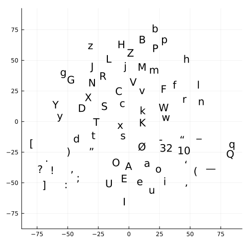
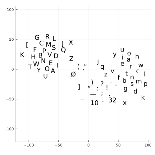
Note that t-SNE is stochastic and each run will give different results.
For the embedding matrix we can see that the model groups all the vowels (a, e, i, o, u) and their capital forms together. It also tends to group the lowercase form and uppercase form together e.g. ‘g’ and ‘G’. The head meanwhile has 3 distinct groups: capital letters, punctuation and lower case letters. It also groups the vowels together.
Perhaps with further training more meaning would be encoded into these vectors.
6.2 Attention scores
We can pass an input to the model and visually inspect the attention scores. To do this we need to alter the transformer functions to return the score as well (including reshaping it as needed). At the top level - the forward pass of the model - these scores should be saved in a vector. Then we can plot them:
using Plots
text = """LYSANDER.
How now, my love? Why is your cheek so pale?
How chance the roses there do fade so fast?"""
tokens = reshape(indexer(collect(text)), :, 1);
X = tokens[1:context_size, :];
X_text = decode(indexer, X[:, 1]);
Y, scores = predict_with_scores(model, X, mask=model.mask); # modified forward pass
s = scores[3][:, :, 3, 1]
s = ifelse.(model.mask, s, NaN)
heatmap(s,
    xticks=(1:context_size, X_text),
    yticks=(1:context_size, X_text),
    yrotation=90,
    aspectratio=:equal,
    xlims=(0.5, n+0.5),
    size=(500, 500),
)
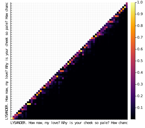
The attention matrices are very sparse. Most tokens only place emphasis on the four or less tokens directly before them. This suggests we could have used a much smaller context length, for example 16 and indeed that does work.
Ideally the model should be learning long range relationships and it is worrying that it is not.
That said, the model does confidently predict that after “How chanc” is an “e”:
using Plots
probs_next = softmax(Y[:, end, 1])
v = length(indexer.vocabulary)
bar(probs_next,
    xticks=(1:v, indexer.vocabulary),
    xlims=(1, v),
    label="",
    ylabel="probabilities",
    xlabel="tokens"
)
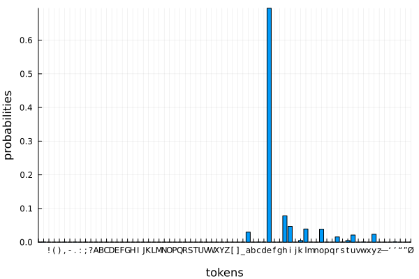
Perhaps with more training the model would give better results.
Conclusion
Thank you for following this tutorial. I hope you now have a working transformer and have much better insight into how they work.
-
The cosine similarity is calculated as $W^TW/ m^T m $ where $m_{1j}=\sqrt{\sum_i W_{ij}^2}$ for each column $j$ in $W$. In code:
using LinearAlgebra function cosine_similarity(W::AbstractMatrix) sim = transpose(W) * W magnitudes = sqrt.(diag(sim)) for i in 1:size(sim, 1) for j in 1:size(sim, 2) sim[i, j] /= magnitudes[i] * magnitudes[j] end end sim end -
In general multiplication is not defined for higher order arrays. But there is a set of multidimensional algebraic objects called tensors where it is. Confusingly, Google named their machine learning framework TensorFlow and calls higher order arrays tensors. So one should differentiate between machine learning tensors and geometric tensors. They are not the same. To give a simple explanation: one can think of geometric tensors as higher order arrays with severe constraints on their entries and operations because they represent geometric objects. These constraints make it harder - not easier - to code higher order arrays as geometric tensors. ↩
-
The design decision is to purposely drop the attention scores in the
TransformerBlock’s forward pass. This is to simplify the code and to not place a bias on the attention. In a typical block theMultiheadAttentionlayer will make up 1/3rd of parameters while the dense layers will make up 2/3rds, so the dense layers are potentially more important. To return the scores you can edit the forward pass for the block and model, or create two new functions entirely. ↩ -
A smarter strategy is to randomly sample passages throughout the text until the desired proportions are reached. ↩