MicroGrad.jl: Part 5 MLP

A series on automatic differentiation in Julia. Part 5 shows how the MicroGrad.jl code can be used for a machine learning framework like Flux.jl. The working example is a multi-layer perceptron trained on the moons dataset.

This is part of a series. The other articles are:

All source code can be found at MicroGrad.jl.

1 Introduction

The previous four sections have developed a minimal automatic differentiation package. The aim of this part is to demonstrate how it can be used as the backbone for a machine learning framework like Flux.jl. In this post we will create a multi-layer perceptron also known as a fully connected neural network. This is an extremely popular and powerful machine learning model. New code will be needed for the forward pass and for some extra rrules. Otherwise, the rest is handled by code from the previous parts.

2 Moons dataset

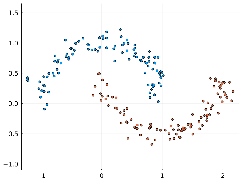
The moons dataset is a toy dataset for testing and visualising classification algorithms. While clearly distinct, the curved nature of the two classes requires a non-linear algorithm to discern them. This was the dataset chosen by Karpathy to demonstrate his micrograd package, and so it will be used here too.

This dataset can be reconstructed in Julia as follows, based on the Scikit-Learn function:

using Random

function make_moons(rng::AbstractRNG, n_samples::Int=100; noise::Union{Nothing, AbstractFloat}=nothing)
    n_moons = floor(Int, n_samples / 2)
    t_min = 0.0
    t_max = π
    t_inner = rand(rng, n_moons) * (t_max - t_min) .+ t_min
    t_outer = rand(rng, n_moons) * (t_max - t_min) .+ t_min
    outer_circ_x = cos.(t_outer)
    outer_circ_y = sin.(t_outer)
    inner_circ_x = 1 .- cos.(t_inner)
    inner_circ_y = 1 .- sin.(t_inner) .- 0.5

    data = [outer_circ_x outer_circ_y; inner_circ_x inner_circ_y]
    z = permutedims(data, (2, 1))
    if !isnothing(noise)
        z += noise * randn(size(z))
    end
    z
end

make_moons(n_samples::Int=100; options...) = make_moons(Random.default_rng(), n_samples; options...)

Creating the moons and labels:

n = 100
X = make_moons(2n; noise=0.1) # 2×200 Matrix 
y = vcat(fill(1, n)..., fill(2, n)...) # 200-element Vector{Int64}

3 Layers

3.1 ReLU

The Rectified Linear Unit (ReLU) is a common activation function in machine learning. It is defined as follows:

\[\text{relu}(x)=\begin{cases} x, & \text{if $x> 0$} \\ 0, & \text{otherwise} \end{cases}\]

This can be realised as a broadcast of the max function:

relu(x::AbstractArray) = max.(0, x)

The derivative is:

\[\frac{\partial \text{relu}}{\partial x}=\begin{cases} 1, & \text{if $x> 0$} \\ 0, & \text{otherwise} \end{cases}\]

In code:

function rrule(::typeof(relu), x::AbstractArray)
    relu_back(Δ) = (nothing, ifelse.(x .> 0, Δ, 0))
    relu(x), relu_back
end

3.2 Dense layer

The fully connected layer equation is:

\[Y_{ij} = a\left(\sum_k (W_{ik}X_{kj} + b_{i}) \right)\]

This is the code from Flux.jl to create this fully connected layer (source):

using Random
struct Dense{M<:AbstractMatrix, B<:AbstractMatrix, F}
    weight::M
    bias::B
    activation::F
end

function (a::Dense)(x::AbstractVecOrMat)
    a.activation(a.weight * x .+ a.bias)
end

Dense((in, out)::Pair; activation=relu) = Dense(glorot_uniform(in, out), zeros(out, 1), activation)

function glorot_uniform(rng::AbstractRNG, fan_in::Int, fan_out::Int)
    scale = sqrt(24 / (fan_in + fan_out))  # 0.5 * sqrt(24) = sqrt(1/4 * 24) = sqrt(6)
    (rand(rng, fan_out, fan_in) .- 0.5) .* scale
end

glorot_uniform(fan_in::Int, fan_out::Int) = glorot_uniform(Random.default_rng(), fan_in, fan_out)

Also add a method to paramaters:

parameters(a::Dense) = (;weight=a.weight, bias=a.bias)

Create and test:

X = rand(2, 4)
layer = Dense(2 => 3; activation=relu)
layer(X) # 3×3 Matrix{Float64}

3.3 Reverse broadcast

Inspect the IR @code_ir layer(X):

1: (%1, %2)
  %3 = Base.getproperty(%1, :activation)
  %4 = Main.:+
  %5 = Base.getproperty(%1, :weight)
  %6 = %5 * %2
  %7 = Base.getproperty(%1, :bias)
  %8 = Base.broadcasted(%4, %6, %7)
  %9 = Base.materialize(%8)
  %10 = (%3)(%9)
  return %10

From part 1 and part 4 we have rrules for getproperty (getfield), matrix multiplication (*) and for the activation (relu). We still need rrules for broadcasted and materialize.

Creating rules for broadcasting in general is complex¹, so instead create a specific rule for the broadcast invoked here:

function rrule(::typeof(Broadcast.broadcasted), ::typeof(+), A::AbstractVecOrMat{<:Real}, B::AbstractVecOrMat{<:Real})
    broadcast_back(Δ) = (nothing, nothing, unbroadcast(A, Δ), unbroadcast(B, Δ))
    broadcast(+, A, B), broadcast_back
end

function unbroadcast(x::AbstractArray, x̄)
    if length(x) == length(x̄)
        x̄
    else
      dims = ntuple(d -> size(x, d) == 1 ? d : ndims(x̄)+1, ndims(x̄))
      dx = sum(x̄; dims = dims)
      check_dims(size(x), size(dx))
      dx
    end
end

function check_dims(size_x, size_dx) # see ChainRulesCore.ProjectTo
    for (i, d) in enumerate(size_x)
        dd = i <= length(size_dx) ? size_dx[i] : 1 # broadcasted dim
        if d != dd 
            throw(DimensionMismatch("variable with size(x) == $size_x cannot have a gradient with size(dx) == $size_dx"))
        end
    end
end

Testing:

X = rand(2, 4)
b = rand(2)
Z, back = rrule(Base.broadcasted, +, X, b) # (2×4 Matrix{Float64}, broadcast_back)
back(ones(2, 4)) # (nothing, nothing, ones(2, 4), [4.0; 4.0;;])

The definition for Base.Broadcast.materialize is:

@inline materialize(bc::Broadcasted) = copy(instantiate(bc))
materialize(x) = x

Hence we need rrules for copy and instantiate (source):

function rrule(::typeof(copy), bc::Broadcast.Broadcasted)
    uncopy(Δ) = (nothing, Δ)
    return copy(bc), uncopy
end

function rrule(::typeof(Broadcast.instantiate), bc::Broadcast.Broadcasted)
    uninstantiate(Δ) = (nothing, Δ)
    return Broadcast.instantiate(bc), uninstantiate
end

Now the pullback for the Dense layer works:

Y, back = pullback(layer, X) # (3×4 Matrix, Pullback)
back(ones(3, 4)) # ((;weight=...,bias=...,activation=nothing), 2×4 Matrix)
Y, back = pullback(m->m(X), layer) # (3×4 Matrix, Pullback)
back(ones(3, 4)) # (nothing, (;weight=...,bias=...,activation=nothing))

3.4 Chain

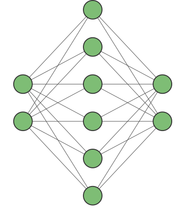
Here is the Flux code to create a generic chain (source):

struct Chain{T<:Tuple}
    layers::T
end
  
Chain(xs...) = Chain(xs)

(c::Chain)(x) = _apply_chain(c.layers, x)

@generated function _apply_chain(layers::Tuple{Vararg{Any,N}}, x) where {N}
  symbols = vcat(:x, [gensym() for _ in 1:N])
  calls = [:($(symbols[i+1]) = layers[$i]($(symbols[i]))) for i in 1:N]
  Expr(:block, calls...)
end

Add a method to parameters:

parameters(c::Chain) = (;layers = map(parameters, c.layers))

We will need an rrule for getindex:

world = Base.get_world_counter()
pr1 = _generate_pullback(world, typeof(_apply_chain), Tuple{typeof(cos), typeof(sin)}, Float64)

It is as follows (source):

function rrule(::typeof(getindex), x::T, i::Integer) where {T<:Tuple}
    function getindex_back_1(Δy)
        dx = ntuple(j -> j == i ? Δy : nothing, length(x))
        return (nothing, (dx...,), nothing)
    end
    return x[i], getindex_back_1
end

Test (compare the results in part 1):

model = Chain(cos, sin)
model(0.9) # 0.5823
z, back = pullback(model, 0.9)
back(1.0) # ((layers=(nothing, nothing),), -0.6368)

Test a multi-layer perceptron:

model = Chain(
    Dense(2 => 16, activation=relu),
    Dense(16 => 16, activation=relu),
    Dense(16=>2, activation=relu)
)
model(X) # 2×4 Matrix
Z, back = pullback(m->m(X), model)  # (2×4 Matrix, Pullback)
back(ones(2, 4)) # (nothing, (layers=((weight=...), (weight=...), (weight=...))))

4 Loss

4.1 Cross entropy

The output of the machine learning model will be a probability $p_j$ for a sample $j$ being in a certain class. This will be compared to a probability for a known label $y_j$, which is either 1 if that sample is in the class or 0 if it is not. An obvious value to maximise is their product:

\[y_j p_j \tag{4.1}\]

with range $[0, 1]$.

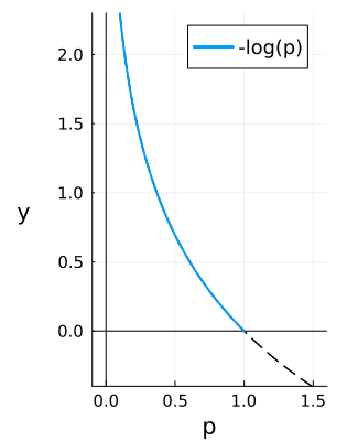
However most machine learning optimisation algorithms aim to minimise a loss. So instead $p_j$ is scaled as $-\log(p_j)$, so that the loss ranges from $[0, \infty)$ with the goal to minimise it at 0. This is called the cross entropy loss:

\[L(p_j, y_j) = -y_j \log(p_j) \tag{4.2} \label{eq:cross_entropy}\]

4.2 Logit cross entropy

The outputs of the neural network are not probabilities but instead a vector of logits containing $N$ real values for $N$ classes. By convention these logits are scaled to a probability distribution using the softmax function:

\[s(x)_i = \frac{e^{x_i}}{\sum_{r=1}^{N} e^{x_r}} \tag{4.3} \label{eq:softmax}\]

Combining equations $\ref{eq:cross_entropy}$ and $\ref{eq:softmax}$ and taking a mean across samples gives the mean logit cross entropy loss:

\[\begin{align} L(x, y) &= -\frac{1}{n}\sum_{j=1}^n \sum_{i=1}^N y_{ij} z_{ij} \\ &= -\frac{1}{n}\sum_{j=1}^n \sum_{i=1}^N y_{ij} \left(x_{ij} - \log\left(\sum_{r=1}^{N} e^{x_{rj}}\right) \right) \end{align} \tag{4.4} \label{eq:logit_cross_entropy}\]

where $z_{ij}$ is the output of the logsoftmax function. Assuming that $y_{ij}$ is 1 for exactly one value of $i$ and 0 otherwise, this can be simplified to:

\[\begin{align} L(x, y) = -\frac{1}{n}\sum_{j=1}^n \left(x_{j} - \log\left(\sum_{r=1}^{N} e^{x_{rj}}\right) \right) \end{align} \tag{4.5} \label{eq:logit_cross_entropy_2}\]

In Julia this can be implemented as follows (source):

using StatsBase
logsoftmax(x::AbstractArray) = x .- log.(sum(exp.(x), dims=1))
function logit_cross_entropy(x::AbstractVecOrMat, y::AbstractVecOrMat)
    mean(-sum(y .* logsoftmax(x), dims=1))
end

According to the multivariable chain rule, the derivative with respect to one logit $x_{ij}$ in the vector for sample $j$ is (gradients come from the main case $k=i$ case as well as the sum in the softmax for $k\neq i$):

\[\begin{align} \frac{\partial L}{\partial x_{ij}} &= \sum_{k=1}^N \frac{\partial L}{\partial z_{kj}} \frac{\partial z_{kj}}{\partial x_{ij}} \\ &= \sum_{k=1}^N \left( -\frac{y_{kj}\Delta}{n} \frac{\partial}{\partial x_{ij}}\left(x_{kj} - \log\left(\sum_{r=1}^{N} e^{x_{rj}}\right) \right) \right) \\ &= \sum_{k=1}^N \left(-\frac{y_{kj} \Delta}{n} \left(\delta_{ij} - \frac{e^{x_{ij}}}{\sum_{r=1}^{N} e^{x_{rj}}} \right) \right) \\ &= -\frac{\Delta}{n} \left(y_{ij} - s(x_j)_{i} \sum_{k=1}^N y_{kj}\right) \end{align} \tag{4.6} \label{eq:back_logitcrossentropy}\]

where $\delta_{ij}$ is the Kronecker delta. Assuming that $y_{kj}$ is 1 for one value of $k$ and 0 otherwise, this simplifies too:

\[\begin{align} \frac{\partial L}{\partial x_{ij}} &= -\frac{\Delta}{n}(y_{ij} - s(x_j)_{i}) \end{align} \tag{4.7} \label{eq:back_logitcrossentropy_2}\]

In Julia this can be implemented as follows (source):

function rrule(::typeof(logsoftmax), x::AbstractArray)
    expx = exp.(x)
    Σ = sum(expx, dims=1)
    function logsoftmax_back(Δ)
        (nothing, Δ .- sum(Δ; dims=1) .* expx ./ Σ)
    end
    x .- log.(Σ), logsoftmax_back
end

function rrule(::typeof(logit_cross_entropy),  x::AbstractVecOrMat, y::AbstractVecOrMat)
    ls, logsoftmax_back = rrule(logsoftmax, x)
    function logit_cross_entropy_back(Δ)
        size_ls = size(ls)
        n = length(size_ls) > 1 ? prod(size(ls)[2:end]) : 1
        ∂x = logsoftmax_back(-y * Δ/n)[2]
        ∂y = -Δ/n .* ls
        return nothing, ∂x , ∂y
    end
    mean(-sum(y .* ls, dims = 1)), logit_cross_entropy_back
end

Testing:

y1, y2 = rand(4), rand(4)
l, back = pullback(logit_cross_entropy, y1, y2) # (2.69, logit_cross_entropy_back)
back(1.0) # (nothing, [0.4,...], [1.37,...] )
X = rand(2, 4) 
Y = [1.0 1.0 0.0 0.0 ; 0.0 0.0 1.0 1.0] # one hot encoded
l, back = pullback(logit_cross_entropy, X, Y)
back(1.0) # (nothing, 2×4 Matrix, 2×4 Matrix)

5 Train and Evaluate

5.1 Train

Create the moons data and labels:

n = 100
X = make_moons(2n; noise=0.1) # 2×200 Matrix 
y = vcat(fill(1, n)..., fill(2, n)...) # 200-element Vector{Int64}

Convert the labels to a one hot presentation:

function onehot(y::AbstractVector, labels)
    num_classes = maximum(labels)
    Y = zeros(num_classes, length(y))
    for (j, label) in enumerate(y)
        Y[label, j] += 1
    end
    Y
end
Y = onehot(y, 1:2)

Create the model:

model = Chain(
    Dense(2 => 16, activation=relu),
    Dense(16 => 16, activation=relu),
    Dense(16=>2, activation=relu)
)

Test the loss function:

l, back = pullback(m->logit_cross_entropy(m(X), Y), model); # (0.69, Pullback{...}(...))
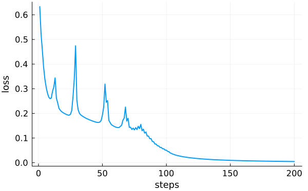
back(1.0) # (nothing, layers=((weight=...),(weight=...),(weight=...),))

Use the exact same gradient_descent! function from part 4:

history = gradient_descent!(
    model, logit_cross_entropy, X, Y
    ; learning_rate=0.9, max_iters=200
)

5.2 Evaluate

Plot the history:

Calculate accuracy:

Y_pred = model(X)
y_pred = vec(map(idx -> idx[1], argmax(Y_pred, dims=1)))
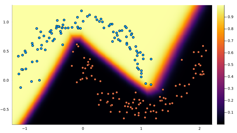
mean(y_pred .== y) # 100%

Plot decision boundary:

using Plots
xmin, xmax = extrema(X[1, :])
ymin, ymax = extrema(X[2, :])
h = 0.01
xrange = (xmin-0.1):h:(xmax+0.1)
yrange = (ymin-0.1):h:(ymax+0.1)

x_grid = xrange' .* ones(length(yrange))
y_grid = ones(length(xrange))' .* yrange
Z = similar(x_grid)
for idx in eachindex(x_grid)
    logits = model([x_grid[idx], y_grid[idx]])
    Z[idx] = softmax(logits)[1]
end
canvas = heatmap(xrange, yrange, Z, size=(800, 500))

Plot points over the boundary:

scatter!(
    X[1, :], X[2, :], color=y, label="", aspectratio=:equal,
    xlims = xlims(canvas),
    ylims = ylims(canvas),
)

The result:

Decision boundary — The probability boundaries of a multi-layer perceptron trained on the moons dataset.

6 Conclusion

That was a long and difficult journey. I hope you understand how automatic differentiation with Zygote.jl works now!

The Zygote.jl code for broadcast has this gem of a comment:

There's a saying that debugging code is about twice as hard as writing it in the first place. So if you're as clever as you can be when writing code, how will you ever debug it?

AD faces a similar dilemma: if you write code that's as clever as the compiler can handle, how will you ever differentiate it? Differentiating makes clever code that bit more complex and the compiler gives up, usually resulting in 100x worse performance.

Base's broadcasting is very cleverly written, and this makes differentiating it... somewhat tricky.

↩

← Previous Post Next Post →

Table of Contents