The Weiler-Atherton polygon clipping algorithm

Description of the Weiler-Atherton polygon clipping algorithm.

Table of Contents

1 Introduction

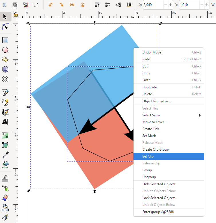
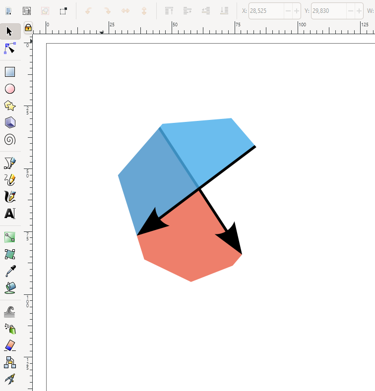
Finding the intersection between two polygons is known as polygon clipping in computer graphics. Polygon clipping is used in computer games and renderers to limit the objects being rendered or while processing shadows. It is also used in vector graphics programs such as Inkscape to alter shapes. Another use is in geospatial sciences to compare the overlap of land areas.

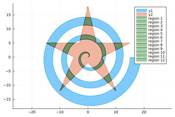
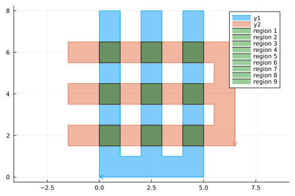
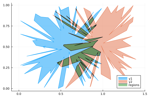
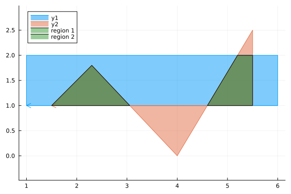
I recently released a PolygonAlgorithms.jl package for Julia. As part of the package I included two algorithms to find the intersection of two polygons. The first is for the intersection of convex polygons developed by Joseph O’Rourke et. al. (1982). This has $\mathcal{O}(n+m)$ time complexity where $n$ and $m$ are the number of vertices of the two polygons. Because the polygons are assumed convex they will have at most one region of intersection. For the general case of concave polygons with multiple regions of intersection I implemented the Weiler-Atherton (1977) polygon algorithm. This algorithm runs in $\mathcal{O}(nm)$ time and can handle a wide variety of polygons, as can be seen above.

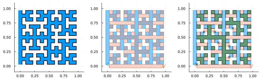
I am particularly proud of the fact that it can handle an extremely complex case of two fractals intersecting each other. This example is from the paper Clipping simple polygons with degenerate intersections (2019). The code for drawing these Hilbert curves can be found here.

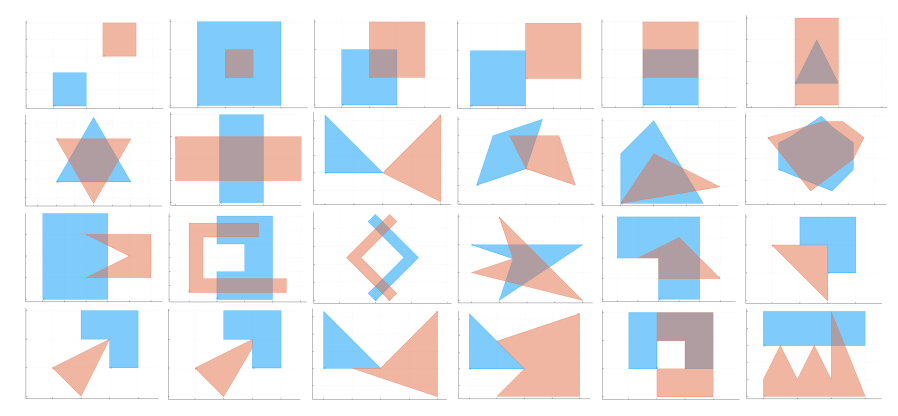
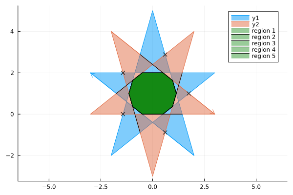
The fact that it can handle complex cases is in part due to extensive testing. There are over 70 unit tests for the algorithm. The figure above shows 24 distinct cases. These are then all run twice with swapped inputs to ensure the function is symmetric. There are further slight variations on the ones shown, such as translations of one of the polygons.

The main code is in this file: intersect_poly.jl. This post will mostly describe the algorithm in pseudo-code and with images so that it can be implemented in any language. The various sections correspond with function names in the code.

Concepts

Finding the intersection of polygons is easy for humans because we can consider the polygon as a whole. However to make an algorithm is challenging since we have to break it up into smaller pieces for a computer.

The main concept behind the Weiler-Atherton algorithm is at any stage we only need 12 pieces of information, six per polygon (for special cases we will need more):

1. The two co-ordinates of each of the two vertices on an edge.
2. The direction of the edge.
3. The fact that the vertices of the polygon as a whole are ordered clockwise.

With points 2 and 3 we can always determine which direction is inside the polygon. (Take a moment to convince yourself of this fact with a pen and paper.)

The Martinez-Rueda Algorithm (2009) is a more recent and more versatile algorithm. It is based on the concept of a vertical line sweep, which gives us more information per step:

For a full explanation of the Martinez-Rueda Algorithm, see this blog post: sean.cm/a/polygon-clipping-pt2. I chose to go with the Weiler-Atherton algorithm because it is simpler.

Limitations

The implementation described here has the following limitations.

1. It does not cater for holes in the polygon. (The original version had an extension for this case.)
2. It can fail completely for self-intersecting polygons. (Extensions for this case do exist.)

In some special cases it will work if only one polygon is self-intersecting but there is no guarantee. It will definitely struggle for two self-intersecting polygons.

The original algorithm could not handle degenerate cases. This version can because of the edge case handling in the Linking intersections section.

2 The algorithm

The Weiler-Atherton algorithm is as follows:

0. Start with two lists of the vertices of polygon 1 and polygon 2 ordered clockwise.
1. Find all the intersections between the edges of polygon 2 with polygon 1.
   1. Insert each intersection into both lists maintaining the clockwise order of points.
   2. Label each intersection as ENTRY or EXIT points depending on if they enter polygon 1 from polygon 2 or exit polygon 1 to polygon 2. Label them as VERTEX if neither. The original algorithm assumed ENTRYs and EXITs alternated after the first intersection; this version does not so it can account for edge cases.
2. Walk through all vertices on polygon 2.
   1. Each time an unvisited ENTRY point is encountered, start recording a region of intersection.
   2. Follow the vertices until an EXIT vertex is encountered, then move to the corresponding vertex on polygon 1.
   3. Continue following the vertices on polygon 1 until an ENTRY vertex is encounted, then move back to the corresponding vertex on polygon 2.
   4. Repeat steps ii and iii until the starting point is encountered. All visited points lie on the region of intersection. Continue along polygon 2.
3. If there is no regions of intersection:
   1. Check if the first non-intersection point of polygon 1 lies in polygon 2. If yes then Polygon 1 lies fully inside polygon 2.
   2. Check if the first non-intersection point of polygon 2 lies in polygon 1. If yes then Polygon 2 lies fully inside polygon 1.
   3. Otherwise they do not intersect.

Step 3 requires a point in polygon algorithm. A walkthrough of that can be found at www.geeksforgeeks.org/how-to-check-if-a-given-point-lies-inside-a-polygon/. This is an $\mathcal{O}(n)$ operation.

The algorithm as a whole can be better understood through a worked example.

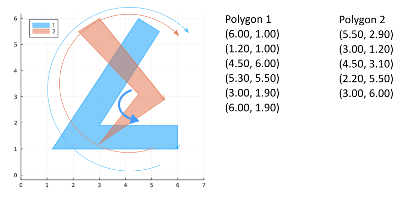
Step 0: First start with two lists of the vertices of the polygons. Globally they should be ordered clockwise although some sections may be counter-clockwise. For example, polygon 1 is ordered clockwise as a whole despite the section (5.3, 5.5), (3.0, 1.9), (6.0, 1.9) being counter-clockwise.

Step 1: find and insert intersections into both lists. Label them as entering or exiting polygon 1 from the perspective of polygon 2. These labels can also be thought of as entering or exiting the intersection regions from the perspective of polygon 2. Create links between the intersection points.

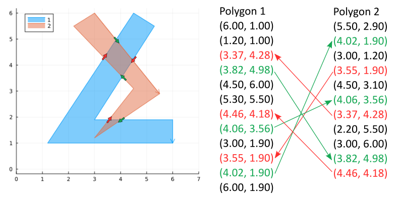
Step 2: walk through the vertices on polygon 2. Whenever an unvisited entry point is found, start walking through a loop following exit/entry points to polygon 1 and back until the starting point is encountered again. These loops are the regions of intersection.

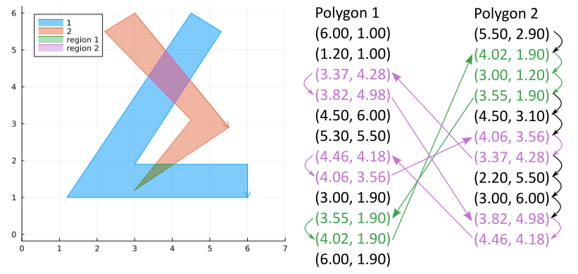
Note that upon entering polygon 1 we walk along the edges on polygon 2 which are inside polygon 1, and upon exiting we walk along the edges of polygon 1 which define the boundary of the region of intersection.

3 Doubly Linked lists

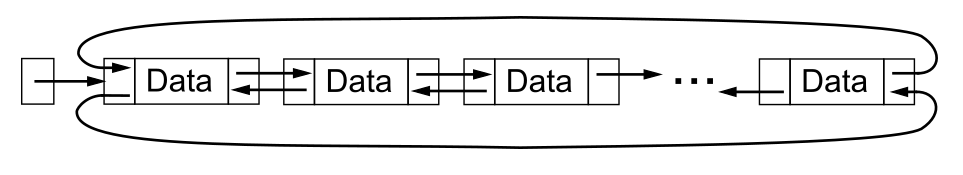
An interesting question is how to create two lists that we can simply insert points in and create links between the two. This problem is solved with doubly linked lists. This is something that I had only ever seen before in coding challenges and interview preparation. This is the first time I’ve had a practical use for it.

Creating doubly linked lists is very language specific. There are many tutorials on it. The rest of this section demonstrates a concrete example with Julia code. To continue with the more generic algorithm, go to the next section.

A first solution might be to have two arrays and a hashmap which keeps track of the links. Here is a toy example which works with characters instead of points:

arr1 = ['a', 'b', 'c']
arr2 = ['d', 'e', 'b', 'f']
links = Dict(2 => 3) # indices1 => indices2
arr1[2] # b
arr2[links[2]] # b

Now insert a new intersection x. We now have to update all the indices:

arr1 = ['a', 'x', 'b', 'c']
arr2 = ['d', 'x', 'e', 'b', 'f']
links = Dict(3 => 4, 2=>2) # indices1 => indices2
arr1[3] # b
arr2[links[3]] # b
arr1[2] # x
arr2[links[2]] # x

That’s a lot of admin.

Consider instead a minimal implementation of a doubly linked list:

mutable struct Node{T}
    data::T
    prev::Node{T}
    next::Node{T}
    function Node(data::T) where T
        node = new{T}(data)
        node.next = node
        node.prev = node
        return node
    end
end

function Node(data::T, prev::Node{T}, next::Node{T}) where T
    node =  Node(data)
    node.prev = prev
    node.next = next
    node
end

struct DoublyLinkedList{T}
    head::Node{T}
end

function Base.push!(list::DoublyLinkedList{T}, data::T) where {T}
    head = list.head
    tail = head.prev
    node = Node(data, tail, head)
    head.prev = node
    tail.next = node
    node
end

function Base.insert!(node::Node{T}, data::T) where {T}
    middle = Node(data, node, node.next)
    node.next.prev = middle
    node.next = middle
    middle
end

Base.iterate(list::DoublyLinkedList) = (list.head.data, list.head.next)
Base.iterate(list::DoublyLinkedList, state::Node) = state == list.head ? nothing : (state.data, state.next)
Base.IteratorSize(::DoublyLinkedList) = Base.SizeUnknown()

Recreate the same lists as before:

list1 = DoublyLinkedList(Node('a'))
node12 = push!(list1, 'b')
node13 = push!(list1, 'c')
list2 = DoublyLinkedList(Node('d'))
node22 = push!(list2, 'e')
node23 = push!(list2, 'b')
node24 = push!(list2, 'f')
links = Dict(node12 => node23)
node12.data # b
links[node12].data # b

Now add in the new node:

node1x = insert!(list1.head, 'x')
node2x = insert!(list2.head, 'x')
push!(links, node1x => node2x)
node12.data # b
links[node12].data # b
node1x.data # x
links[node1x].data # x

Note how we didn’t have to update the old links. The underlying pointers still point to the same data, which is why we went to all this effort.

Lastly we can collect the lists to recreate the arrays as before:

collect(list1) # ['a','x','b','c']
collect(list2) # ['d','x','e','b','f']

4 Find and insert intersections

4.1 Finding intersections

A straightforward way to find intersections is to compare all pairs of edges. There are ${nm}$ pairs so this is an $\mathcal{O}(nm)$ algorithm.

Find intersections
for edge$_2$ $\leftarrow$ original(polygon$_2$) do:
$\quad$ for edge$_1$ $\leftarrow$ original(polygon$_1$) do:
$\quad\quad$ $p \leftarrow$ intersect(edge$_1$, edge$_2$)
$\quad\quad$ if $p$
$\quad\quad\quad$ node$_1$ $\leftarrow$ insert_in_order(polygon$_1$, $p$)
$\quad\quad\quad$ node$_2$ $ \leftarrow$ insert_in_order(polygon$_2$, $p$)
$\quad\quad\quad$ link_intersections!(node$_1$,node$_2$)
return polygon$_1$, polygon$_2$

A faster algorithm is the Bently-Ottman algorithm which is utilised in the Martinez-Rueda algorithm.

4.2 Calculating intersections

Calculating the intersection of two edges is an elementary exercise in algebra. Here is one possible methodology.

Define a line as: \(ax+by = c\)

A segment $\{(x_1, y_1), (x_2, y_2)\}$ can be fit to a line with:

The intersection between two lines can be calculated with linear algebra:

If the determinant $\Delta = a_1 b_2 - a_2 b_1=0$ then there is no intersection. Otherwise the resulting point must lie on both segments. This condition is satisfied when $\min(x_1, x_2) \leq x \leq \max(x_1, x_2)$ and $\min(y_1, y_2) \leq y \leq \max(y_1, y_2)$ for both segments.

4.3 Inserting intersections in order

The intersections have to be inserted maintaining the clockwise order. If there is one intersection on the edge the new point can be automatically placed between the tail and the head of the edge. Otherwise if there are multiple intersections on the edge (see the example) then we need to determine which intersection is placed first. The basic idea is to check that the distance from the current vertex to the intersection is less than the distance from the current vertex to the next vertex. If not, advance one vertex forward (on to an existing intersection point) and try again. We also need to check if the intersection was already inserted or equivalently, the same as an original vertex of the polygon.

Insert intersection in order
inputs: $p$, edge
tail, head $\leftarrow$ edge
$s \leftarrow$ tail
while $s \neq$ head
$\quad$ if $|p - s| =0$
$\quad\quad$ return $s$
$\quad$ else if $|s_+ - p| =0$
$\quad\quad$ return $s_+$
$\quad$ else if $|p - s | < |s_+ - s|$
$\quad\quad$ break
$\quad$ $s\leftarrow s_+$
$s_+\leftarrow $insert($s$, $p$)
return $s_+$

Here $s_+$ refers to the vertex after $s$.

5 Linking intersections

5.1 Half-planes

A major aspect of the algorithm is defining if intersection points are entry or exit points. One possible way is to check if the point after the intersection region lies in the polygon. A problem with that idea is these checks are slow: $\mathcal{O}(n)$.

A much quicker way to do this is with something called a half-plane. It only requires knowing the edge, the point and that the polygons are clockwise. This check is immediate: $\mathcal{O}(1)$.

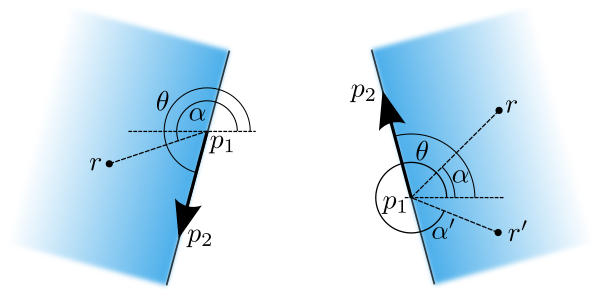
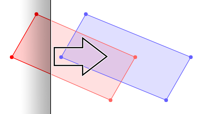
The half-plane of an edge is defined as the plane stretching from that edge into the polygon into infinity, above, below and to the side of the edge. Because the polygons are always clockwise, a ray $(p_1, r)$ with angle $\alpha$ will lie outside the half-plane of $(p_1, p_2)$ with angle $\theta$ if:

For it to lie in the half plane it therefore requires that:

The angles can be calculated directly with $\arctan$. However a more efficient formula can be derived by noting that both conditions are satisfied when:

The derivation uses the double angle formula for $\sin$ and the identity $\sin(\pi +\beta) =-\sin\beta$.

More detail: cross product derivation ⇩

So to determine if an edge is entering or leaving polygon 1, we can take the next vertex of polygon 2 after the intersection - the head - and use equation $\ref{eq:half-plane}$ to determine if it is inside (entering) or outside (exiting) the half-plane of the edge of polygon 1. This works well in most scenarios.

Complexity comes in that sometimes the head and/or tail of the edge lies on the edge of polygon 1. The half-plane formula is a strict inequality because it does not cater for the case of a point lying on the dividing line. These are edge cases that need to be handled separately. They are edge cases in the sense that there are literal edges involved, but also in the broader sense of algorithms in that they are unusual cases that lie on the boundary between different scenarios and which leave us with choices on how to handle them. Most of the test cases are for these situations.

The next two subsections explore the edge cases.

5.2 Edge intersections

An edge intersection happens when a vertex of polygon 2 lies on an edge of polygon 1.

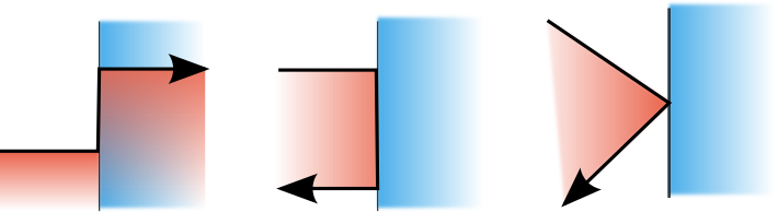
There are 6 case of edge intersections:

1. Polygon 2 first intersects polygon 1 on an edge and then enters polygon 1.
2. Polygon 2 only intersects polygon 1 on edges.
3. Polygon 2 only intersects polygon 1 at a single point.
4. The first three cases but the edges of polygon 2 are inside polygon 1. These cases do not count as entering or exiting.

We have a choice to count theses cases intersections or not. For a graphical application they might not be relevant. However I wanted my algorithm to return the edge intersections if there was only an edge intersection or a point if there was only a point intersection. Therefore my code counts hitting an edge of polygon 1 as entering polygon 1 if the tail of edge 2 is not in polygon 1. The case of exiting is dealt with separately. Here the rule is: polygon 2 is exiting polygon 1 if the head of edge 2 is not in polygon 1.

In the case of the point intersection it will be an entry followed immediately by an exit. This should then be changed to a vertex intercept.

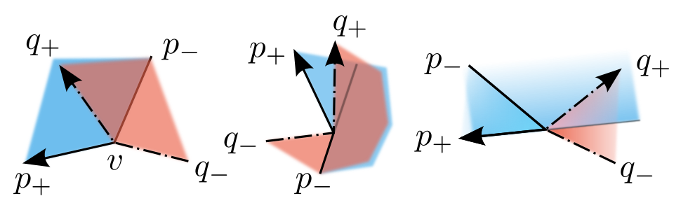
5.3 Vertex intersections

A vertex intersection happens when a vertex of polygon 2 lies on a vertex of polygon 1. For example:

This can be conceptually thought of as a “bent” edge. There are several cases are which correspond to the cases already profiled for “straight” edges:

1. The polygons cross over each other at the common vertex. This is either an ENTRY or EXIT.
2. One polygon is inside/outside the other polygon and they touch at common vertex (VERTEX).
3. The polygons have overlapping edges which touch at the common vertex. This is either an ENTRY or EXIT or a shared segment on a longer segment (VERTEX).

There are three consecutive points on each polygon: the previous tail $p_-$, the intersection point/vertex $p$ and the next head $p_+$. The letter $p$ or $q$ denotes the polygon. Note that $v\equiv p \equiv q$. The algorithm is then as follows:

Link vertex intersections
inputs: $v$, $p_{-}$, $p_{+}$, $q_{-}$, $q_{+}$
edge$_{1-}$ $\leftarrow (p_{-}, v)$
edge$_{1+}$ $\leftarrow (v, p_{+})$
prev2_on_edge1 $\leftarrow$ has_edge_overlap($v$, $p_{-}$, $p_{+}$, $q_{-}$)
next2_on_edge1 $\leftarrow$ has_edge_overlap($v$, $p_{-}$, $p_{+}$, $q_{+}$)
tail2_in_1 $\leftarrow$ in_plane(($p_{-}$, $v$, $p_{+}$), $q_{-}$)
head2_in_1 $\leftarrow$ in_plane(($p_{-}$, $v$, $p_{+}$), $q_{+}$)
tail2_in_1 $\leftarrow$ tail2_in_1 $\cup$ prev2_on_edge1
head2_in_1 $\leftarrow$ head2_in_1 $\cup$ next2_on_edge1
if tail2_in_1 = head2_in_1
$\quad$ return VERTEX
else
$\quad$ return ENTRY if head2_in_1 else EXIT

This little algorithm was arrived at after much pain, trial and error.

The half-plane equation $\ref{eq:half-plane}$ is not enough to tell if a point lies inside the polygon. If the point lies in both half-planes then it is definitely in the polygon and if it lies outside both then it is definitely outside. However if it lies in one then it can be either inside or outside.

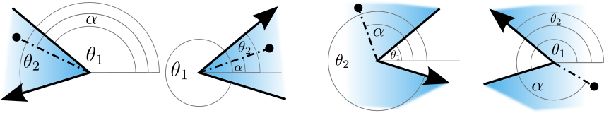
Instead it is better to analyse the angles for a definitive answer. Keeping in mind that the planes need to be clockwise of the edges, there are only two cases to account for. The first is that the tail edge angle $\theta_1$ is less than the leading edge angle $\theta_2$, and the second that it is greater. Then a point with angle $\alpha$ will lie inside if:

The angle from a point $(x, y)$ to the vertex $v$ is calculated as:

The resulting angles should be in the range $[0, 2\pi]$. Most programming languages have an atan2 function which returns in the range $[-\pi, \pi]$. This function with the negative values shifted by $+2\pi$ will have the desired range.

5.4 Edge overlap

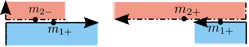
The segment midpoint from each point $(x,y)$ to the vertex $v$ is calculated as:

To check if a specific edge overlaps with one of the other polygon’s edges requires checking if (1) this midpoint lies on the other edge and/or (2) if the other edge’s midpoint lies on this edge. The one edge might be significantly shorter so both might not be true. We do this for both the head and the tail edges of the other polygon to account for the direction being the same as or opposite to the current edge.

To fully check overlap we have to do this for both edges of polygon 2. So 2 checks per 2 directions per 2 edges is 8 checks in total.

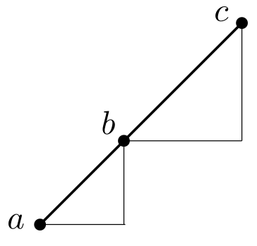
Determining if a point $b$ lies on a segment $\mathbf{ac}$ requires that the cross product $(\mathbf{c}-\mathbf{b}) \times (\mathbf{b}-\mathbf{a})$ is $0$ and that $b$ lies within the bounds $\min(a_x, c_x) \leq b_x \leq \max(a_x, c_x)$ and $\min(a_y, c_y) \leq b_y \leq \max(a_y, c_y)$. Equivalently, the lines have the same gradient and $b$ lies within those bounds.

6 Walk linked lists

Most of the complexity is in creating the linked lists. Once they are made the rest is easy.

First an outer function for walking through all the points on polygon 2:

Walk linked lists
$s_0$: polygon head
regions $\leftarrow $ Array()
visited $\leftarrow \emptyset$
$s \leftarrow s_0$
while $s$
$\quad$ if ($s \notin$ visited) $\cap$ (type($s)=$ENTRY)
$\quad\quad$ region, visited_nodes $\leftarrow$ walk_loop($s$)
$\quad\quad$ regions $\leftarrow$ regions + region
$\quad\quad$ visited $\leftarrow$ visited + points(visited_nodes)
$\quad s \leftarrow$ if $s_+=s_0$ then NULL else $s_+$
return regions

Then an inner function for walking loops between polygon 1 and polygon 2:

Walk loop
$s_0$: node
loop $\leftarrow [s_0]$
visited $\leftarrow \{ s_0 \}$
$s \leftarrow s_{0+}$
while $s \neq s_0$
$\quad$ loop $\leftarrow$ loop $+ s$
$\quad$ if ($s \in$ visited) $\cap$ (type($s$) $\neq$ VERTEX)
$\quad\quad$ ERROR "Cycle detected at node $s$"
$\quad$ visited $\leftarrow$ visited $+ s$
$\quad$ if has_link($s$) $\cap$ (type($s$) $\neq$ VERTEX)
$\quad\quad$ $s \leftarrow$ link($s$)
$\quad$ $s \leftarrow s_+$
return loop, visited

The cycle detection code is important. Despite the best effort so far, there are still some cases where this code could result in infinite loops because of repeated nodes.

My code currently raises a warning instead of an error. I recognise that a message of “cycle detected at node x” is not very informative if you don’t know the underlying algorithm. However at least it gives a clear indication of where the problem lies if you do.

Conclusion

This algorithm performs very well and I am quite satisfied with it.

There are some other smaller details that I have glossed over. For example, floating point numerical errors need to be accounted for. One solution I used is a custom PointSet implementation where all entries are rounded to 6 decimal places before being hashed into the set’s dictionary. That way $s \in \text{visited}$ will not fail if one point is slightly different to another, but they both represent the same intersection point.

There are further extensions for self-intersecting polygons which I may implement in the future.

I am considering implementing the Martinez-Rueda algorithm because it readily handles self-intersecting polygons and can also do unions, differences and XOR.