A random forest classifier in 360 lines of Julia code. It is written from (almost) scratch.
This post is a copy of my previous post on a random forest classifier written in Python, except the code and images were created with Julia. Some explanations have also been changed. As an exercise principle, no code or image was generated with PyCall. The goal of this post is to show that equivalent code can be created with Julia, except this code is 9x faster.
I recently learnt about Random Forest Classifiers/Regressors. It is a supervised machine learning technique that performs well on interpolation problems. It was formally introduced in 2001 by Leo Breiman. They are much easier to train and much smaller than the more modern, but more powerful, neural networks. They are often included in major machine learning software and libraries, including R and Scikit-learn.
There are many article describing the theory behind random forests. See for example 1 or 2. By far the best and most detailed explanation I have seen is given by Jeremy Howard in his FastAI course. A few sources describe how to implement them from scratch, such as 3 or 4.
My aim here is to describe my own implementation of a random forest from scratch for teaching purposes. It is assumed the reader is already familiar with the theory. I hope this post will clarify in-depth questions. The first version was based on Python code in the FastAI course. The full code can be accessed at my Github repository.
Having been inspired by Jeremy Howard’s teaching methods, I will present this post in a top-down fashion.
First I’ll introduce two datasets and show how the random forest classifier can be used on them.
Next, I’ll describe the high level AbstractClassifier type, then the two concrete subtypes based off it,
RandomForestClassifier and DecisionTreeClassifier. Lastly I’ll describe the BinaryTree struct that is used in the DecisionTreeClassifier.
All code is also explained top-down.
Practice Data Sets
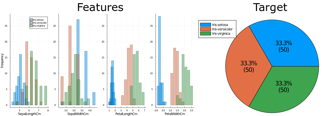
The Iris flower dataset
The Iris flower dataset is commonly used for beginner machine learning problems. The full dataset can be found on Kaggle at www.kaggle.com/arshid/iris-flower-dataset. It consists of 150 entries for 3 types of iris plants, and 4 features: sepal length and width, and petal length and width.1
The variable distributions are as follows:
Based on these, a simple baseline model can be developed:
- If PetalLength < 2.5cm, class is Setosa.
- Else determine scores score1 and score2 as follows:
- score1: add 1 for each of the following that is true:
- 2.5cm < PetalLength ≤ 5.0cm
- 1.0cm≤ PetalWidth ≤ 1.8cm
- score2: add 1 for each of the following that is true:
- 7.0cm≤ SepalLength
- 3.5cm≤ SepalWidth
- 5.0cm≤ PetalLength
- 1.7cm< PetalWidth
- score1: add 1 for each of the following that is true:
- If score1 > score2, classify as Veriscolor. If score1 < score2, classify as Virginica. If score1 = score2, leave unknown, or classify at random.
This simple strategy guarantees that 140 samples, which is 93.3% of the samples, will be correctly classified.
I used my code to make a random forest classifier with the following parameters:
forest = RandomForestClassifier(n_trees=10, bootstrap=True, max_features=4, min_samples_leaf=3)
I randomly split the data into 120 training samples and 30 test samples. The forest took 0.01 seconds to train. It had trees with depths in the range of 2 to 4, and 31 leaves in total. It misclassified one sample in the training and two in the test set, for an accuracy of 99.2% and 96.7% respectively. This is a clear improvement on the baseline.
This is one such tree in the forest:
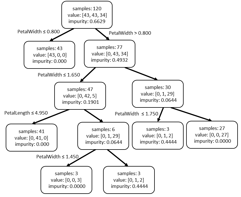
The value is the number of samples in each class in that node. The impurity is a measure of the mix of classes in the node. A pure node has only 1 type of class and 0 impurity. More will be explained on this later. The split is the rule for determining which values go to the left or right child.
Universal Bank loans
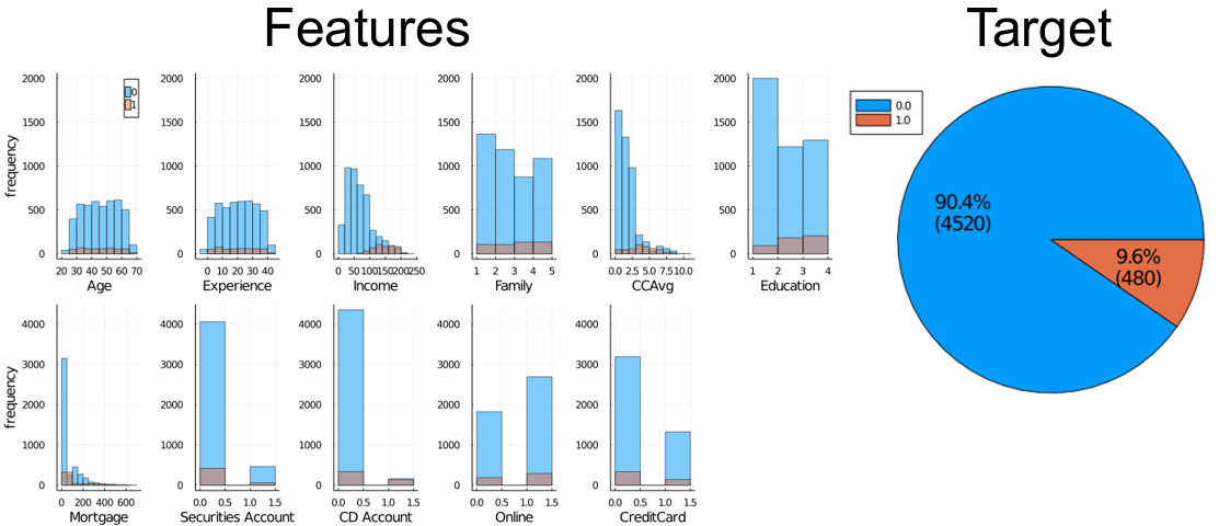
The next dataset I tested was the Bank_Loan_Classification dataset available on Kaggle at www.kaggle.com/sriharipramod/bank-loan-classification/. This dataset has 5000 entries with 11 features. The target variable is “Personal Loan”, and it can be 0 or 1. (Personal Loan approved? Or paid? I don’t know.)
The variable distributions are as follows:
The Pearson correlation coefficients between the features and the target variables are:
| Feature | Correlation | |
|---|---|---|
| 1 | Income | 0.5025 |
| 2 | CCAvg | 0.3669 |
| 3 | CD Account | 0.3164 |
| 4 | Mortgage | 0.1421 |
| 5 | Education | 0.1367 |
| 6 | Family | 0.0614 |
| 7 | Securities Account | 0.0220 |
| 8 | Experience | -0.0074 |
| 9 | Age | -0.0077 |
| 10 | Online | 0.0063 |
| 11 | CreditCard | 0.0028 |
For the baseline model, we could always predict a 0, and claim an accuracy of 90.4%. But this has an F1 score of 0.2 A better baseline is simply to have: 1 if Income > 100 else 0. This has an accuracy of 83.52% and a F1 score of 0.516 over the whole dataset.
I used my code to make a random forest classifier with the following parameters:
forest = RandomForestClassifier(n_trees=20, bootstrap=True, max_features=3, min_samples_leaf=3)
I randomly split the data into 4000 training samples and 1000 test samples and trained the forest on it.
The forest took about 0.90 seconds to train.
The trees range in depth from 11 to 16, with 43 to 120 leaves. The total number of leaves is 1696.
The training accuracy is 99.67% and the test accuracy is 98.60%. The F1 score for the test set is 0.92.
This is a large improvement on the baseline, especially for the F1 score.
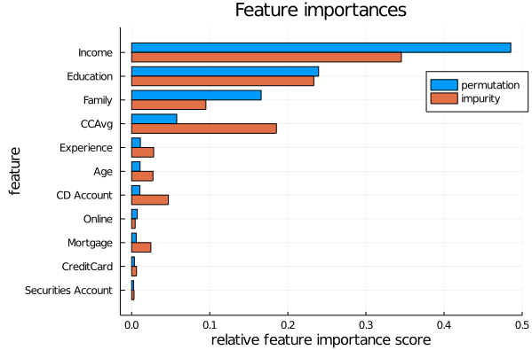
We can inspect the random forest and calculate a feature importance for each feature. The following graph is a comparison between two types of (normalised) feature importances. The orange bars are based on how much that feature contributes to decreasing the impurity levels in the tree. The blue bars are based on randomly scrambling that feature column, and recording how much this decreases the overall accuracy of the model. More detail on these calculations will be given later.
Code
TreeEnsemble
This is a very short file which defines a module TreeEnsemble, includes all the other code, and exports some functions and types for external use.
It also extends Base.size with two new methods.
module TreeEnsemble

export  AbstractClassifier, predict, score, fit!, perm_feature_importance,
        # binary tree
        BinaryTree, add_node!, set_left_child!, set_right_child!, get_children,
        is_leaf, nleaves, find_depths, get_max_depths,
        # Decision Tree Classifier
        DecisionTreeClassifier, predict_row, predict_batch, predict_prob,
        feature_importance_impurity, print_tree, node_to_string,
        # Random Forest Classifier
        RandomForestClassifier,
        # utilities
        check_random_state, split_data, confusion_matrix, calc_f1_score

include("RandomForest.jl")

end
AbstractClassifier
The first step is to create a high level AbstractClassifier. We would like certain methods to always be associated with this struct, such as predict and fit!.
Unfortunately there is no way to force inheritance in Julia (like one can do with the keyword virtual in C++).
The best we can do is make dummy functions that will throw errors if they are not implemented in concrete subtypes of AbstractClassifier.
using DataFrames
using Statistics

abstract type AbstractClassifier end

function predict(classifier::AbstractClassifier, X::DataFrame)
    throw("predict not implemented for classifier of type $(typeof(classifier))")
end

function fit!(classifier::AbstractClassifier, X::DataFrame, Y::DataFrame)
    throw(error("fit! not implemented for classifier of type $(typeof(classifier))"))
end
Some functions can be defined to act on all subtypes of AbstractClassifier. These are independent of the specifics of the classifier.
For example, here is a score function:
function score(classifier::AbstractClassifier, X::DataFrame, Y::DataFrame)
    y_pred = predict(classifier, X)
    return count(y_pred .== Y[:, 1]) / size(Y, 1)
end
As long as a Classifier implements the predict function, we can safely pass it to the above score function.
Another such function is the perm_feature_importance, which can be found in the repository.
A nice to have is throwing common errors for all classifiers. For example, if the classifier has not yet been fitted to data, we can throw a NotFittedError:
import Base: showerror

struct NotFittedError <: Exception
    var::Symbol
end

Base.showerror(io::IO, e::NotFittedError) = print(io, e.var, " has not been fitted to a dataset. Call fit!($(e.var), X, Y) first")
RandomForestClassifier
The next step is create the RandomForestClassifier. Initialising an instance of the struct only sets the internal parameters and does not fit the data.
All parameters have to be in the initial struct, so some of these are set to nothing until a dataset is fitted.3
using Random
using CSV, DataFrames, Printf

include("DecisionTree.jl")

mutable struct RandomForestClassifier{T}  <: AbstractClassifier
    #internal variables
    n_features::Union{Int, Nothing}
    n_classes::Union{Int, Nothing}
    features::Vector{String}
    trees::Vector{DecisionTreeClassifier}
    feature_importances::Union{Vector{Float64}, Nothing}

    # external parameters
    n_trees::Int
    max_depth::Union{Int, Nothing}
    max_features::Union{Int, Nothing} # sets n_features_split
    min_samples_leaf::Int
    random_state::Union{AbstractRNG, Int}
    bootstrap::Bool
    oob_score::Bool
    oob_score_::Union{Float64, Nothing}

    RandomForestClassifier{T}(;
            n_trees=100,
            max_depth=nothing,
            max_features=nothing,
            min_samples_leaf=1,
            random_state=Random.GLOBAL_RNG,
            bootstrap=true,
            oob_score=false
        ) where T = new(
            nothing, nothing, [], [], nothing, n_trees,
            max_depth,
			max_features,
			min_samples_leaf,
			check_random_state(random_state),
			bootstrap,
			oob_score,
			nothing
            )
end
The type T can be determined from the training dataset.
But most of the time it will be Float64, so we can make an outer constructor to make this type the default:
RandomForestClassifier(;n_trees=100, max_depth=nothing, max_features=nothing, min_samples_leaf=1, random_state=Random.GLOBAL_RNG,
        bootstrap=true, oob_score=false
    ) = RandomForestClassifier{Float64}(n_trees=n_trees, mx_depth=max_depth, max_features=max_features, min_samples_leaf=min_samples_leaf,
        random_state=random_state, bootstrap=bootstrap, oob_score=oob_score)
I’ve shown an include for “DecisionTree.jl” which I’ll describe later. “DecisionTree.jl” itself includes “Classifier.jl” and “Utilities.jl” so we don’t need to include them here.4
The supervised learning is done by calling the fit!() function.
This creates each tree one at a time.
Most of the heavy lifting is done by other functions.
Afterwards, it sets attributes including the feature importances and the out-of-bag (OOB) score.
The random state is saved before each tree is made, because this can be used to exactly regenerate the random indices for the OOB score.
This is much more memory efficient than saving the whole list of random indices for each tree.
function fit!(forest::RandomForestClassifier, X::DataFrame, Y::DataFrame)
    @assert size(Y, 2) == 1 "Output Y must be an m x 1 DataFrame"

    # set internal variables
    forest.n_features = size(X, 2)
    forest.n_classes = size(unique(Y), 1)
    forest.features = names(X)
    forest.trees = []

    # create decision trees
    rng_states = typeof(forest.random_state)[]  # save the random states to regenerate the random indices for the oob_score
    for i in 1:forest.n_trees
        push!(rng_states, copy(forest.random_state))
        push!(forest.trees, create_tree(forest, X, Y))
    end

    # set attributes
    forest.feature_importances = feature_importance_impurity(forest)
    if forest.oob_score
        if !forest.bootstrap
            println("Warning: out-of-bag score will not be calculated because bootstrap=false")
        else
            forest.oob_score_ = calculate_oob_score(forest, X, Y, rng_states)
        end
    end

    return
end
The create_tree() function is called by fit!(). It randomly allocates samples, and creates a DecisionTreeClassifier with the same parameters as the RandomForestClassifier.
It then dispatches the heavy lifting to the DecisionTreeClassifier’s fit!() function.
function create_tree(forest::RandomForestClassifier, X::DataFrame, Y::DataFrame)
    n_samples = nrow(X)

    if forest.bootstrap # sample with replacement
        idxs = [rand(forest.random_state, 1:n_samples) for i in 1:n_samples]
        X_ = X[idxs, :]
        Y_ = Y[idxs, :]
    else
        X_ = copy(X)
        Y_ = copy(Y)
    end

	T = typeof(forest).parameters[1] # use the same type T used for the forest
    new_tree = DecisionTreeClassifier{T}(
            max_depth = forest.max_depth,
            max_features = forest.max_features,
            min_samples_leaf = forest.min_samples_leaf,
            random_state = forest.random_state
    )
    fit!(new_tree, X_, Y_)

    return new_tree
end
The prediction of the forest is done through majority voting. In particular, a ‘soft’ vote is done, where each tree’s vote is weighted by its probability prediction per class. The final prediction is therefore equivalent to the class with the maximum sum of probabilities.
function predict_prob(forest::RandomForestClassifier, X::DataFrame)
    if length(forest.trees) == 0
        throw(NotFittedError(:forest))
    end
    probs = zeros(nrow(X), forest.n_classes)
    for tree in forest.trees
        probs .+= predict_prob(tree, X)
    end
    return probs
end

function predict(forest::RandomForestClassifier, X::DataFrame)
    probs = predict_prob(forest, X)
    return mapslices(argmax, probs, dims=2)[:, 1]
end
If bootstrap=true that means each tree is only trained on a subset of the data.
The out-of-bag score can then be calculated as the prediction for each sample based on the trees it was not used to train.
It is a useful measure of the accuracy of the training.
For sampling with replacement, where the sample size is the size of the dataset, we can expect on average 63.2% of samples to be unique.5
This means that per tree 36.8% samples are out-of-bag and can be used to calculate the OOB score.
function calculate_oob_score(
    forest::RandomForestClassifier, X::DataFrame, Y::DataFrame,
    rng_states::Vector{T}) where T <: AbstractRNG
    n_samples = nrow(X)
    oob_prob  = zeros(n_samples, forest.n_classes)
    oob_count = zeros( n_samples)
    for (i, rng) in enumerate(rng_states)
        idxs = Set([rand(forest.random_state, 1:n_samples) for i in 1:n_samples])
        # note: expected proportion of out-of-bag is 1-exp(-1) = 0.632...
        # so length(row_oob)/n_samples ≈ 0.63
        row_oob =  filter(idx -> !(idx in idxs), 1:n_samples)
        oob_prob[row_oob, :] .+= predict_prob(forest.trees[i], X[row_oob, :])
        oob_count[row_oob] .+= 1.0
    end
    # remove missing values
    valid = oob_count .> 0.0
    oob_prob = oob_prob[valid, :]
    oob_count = oob_count[valid]
    y_test = Y[valid, 1]
    # predict out-of-bag score
    y_pred = mapslices(argmax, oob_prob./oob_count, dims=2)[:, 1]
    return mean(y_pred .==  y_test)
end
The final function in RandomForestClassifier calculates the impurity based feature importance. It does so by finding the mean of the feature importances in each tree.
The detail behind these will be delayed to the next section.
function feature_importance_impurity(forest::RandomForestClassifier)
    if length(forest.trees) == 0
        throw(NotFittedError(:forest))
    end
    feature_importances = zeros(forest.n_trees, forest.n_features)
    for (i, tree) in enumerate(forest.trees)
        feature_importances[i, :] = tree.feature_importances
    end
    return mean(feature_importances, dims=1)[1, :]
end
DecisionTreeClassifier
Each DecisionTreeClassifier is a stand-alone estimator. Most of the complexity is actually in this class. So far, the RandomForestClassifier has mostly accumulated the results of it.
using Random
using CSV, DataFrames
using Printf
import Base: size

include("Classifier.jl")
include("Utilities.jl")

mutable struct DecisionTreeClassifier{T} <: AbstractClassifier
    #internal variables
    num_nodes::Int
    binarytree::BinaryTree
    n_samples::Vector{Int} # total samples per each node
    values::Vector{Vector{Float64}} # samples per class per each node. Float64 to speed up calculations
    impurities::Vector{Float64}
    split_features::Vector{Union{Int, Nothing}}
    split_values::Vector{Union{T, Nothing}} #Note: T is the same for all values
    n_features::Union{Int, Nothing}
    n_classes::Union{Int, Nothing}
    features::Vector{String}
    feature_importances::Union{Vector{Float64}, Nothing}

    # external parameters
    max_depth::Union{Int, Nothing}
    max_features::Union{Int, Nothing} # sets n_features_split
    min_samples_leaf::Int
    random_state::Union{AbstractRNG, Int}

    DecisionTreeClassifier{T}(;
        max_depth=nothing,
        max_features=nothing,
        min_samples_leaf=1,
        random_state=Random.GLOBAL_RNG
        ) where T = new(
            0, BinaryTree(), [], [], [], [], [], nothing, nothing, [], nothing,
            max_depth, max_features, min_samples_leaf, check_random_state(random_state)
            )
end
The important variables are stored in arrays. The binary tree structure is stored in a separate class, BinaryTree. A node ID is used to retrieve elements from the BinaryTree. As long as we keep track of these node IDs, we can fully abstract the complexity of the BinaryTree.
As with the RandomForestClassifier, we can set the default type for the variable T to be Float64:
DecisionTreeClassifier(; max_depth=nothing, max_features=nothing, min_samples_leaf=1, random_state=Random.GLOBAL_RNG
	) = DecisionTreeClassifier{Float64}(max_depth=max_depth, max_features=max_features, min_samples_leaf=min_samples_leaf,
		random_state=check_random_state(random_state)
    )
The fit! function is again separate to initialisation.
It starts a recursive call to split_node!() which grows the tree until a stopping criterion is reached.
function fit!(tree::DecisionTreeClassifier, X::DataFrame, Y::DataFrame)
    @assert size(Y, 2) == 1 "Output Y must be an m x 1 DataFrame"

    # set internal variables
    tree.n_features = size(X, 2)
    tree.n_classes = size(unique(Y), 1)
    tree.features = names(X)

    # fit
    split_node!(tree, X, Y, 0)

    # set attributes
    tree.feature_importances = feature_importance_impurity(tree)

    return
end
The function split_node!() does many different actions:
- Increases the sizes of the internal arrays and BinaryTree.
- Calculates the values and impurity of the current node.
- Randomly allocates a subset of features. Importantly, this is different per split. If the whole tree was made from the same subset of features, it is likely to be 'boring' and not that useful.
- Makes a call to `find_better_split()` to determine the best feature to split the node on. This is a greedy approach because it expands the tree based on the best feature right now.
- Creates children for this node based on the best feature for splitting.
function count_classes(Y, n::Int)
    counts = zeros(n)
    for entry in eachrow(Y)
        counts[entry[1]] += 1.0
    end
    return counts
end

function set_defaults!(tree::DecisionTreeClassifier, Y::DataFrame)
    values = count_classes(Y, tree.n_classes)
    push!(tree.values, values)
    push!(tree.impurities, gini_score(values))
    push!(tree.split_features, nothing)
    push!(tree.split_values, nothing)
    push!(tree.n_samples, size(Y, 1))
    add_node!(tree.binarytree)

end

function split_node!(tree::DecisionTreeClassifier, X::DataFrame, Y::DataFrame, depth::Int)
    tree.num_nodes += 1
    node_id = tree.num_nodes
    set_defaults!(tree, Y)
    if tree.impurities[node_id] == 0.0
        return # only one class in this node
    end

    # random shuffling ensures a random variable is used if 2 splits are equal or if all features are used
    n_features_split = isnothing(tree.max_features) ? tree.n_features : min(tree.n_features, tree.max_features)
    features = randperm(tree.random_state, tree.n_features)[1:n_features_split]

    # make the split
    best_score = Inf
    for i in features
        best_score = find_better_split(i, X, Y, node_id, best_score, tree)
    end
    if best_score == Inf
        return # no split was made
    end

    # make children
    if isnothing(tree.max_depth) || (depth < tree.max_depth)
        x_split = X[:, tree.split_features[node_id]]
        lhs = x_split .<= tree.split_values[node_id]
        rhs = x_split .>  tree.split_values[node_id]
        set_left_child!(tree.binarytree, node_id, tree.num_nodes + 1)
        split_node!(tree, X[lhs, :], Y[lhs, :], depth + 1)
        set_right_child!(tree.binarytree, node_id, tree.num_nodes + 1)
        split_node!(tree, X[rhs, :], Y[rhs, :], depth + 1)
    end

    return
end
find_better_split() is the main machine learning function. It is not surprisingly the slowest function in this code and the main bottleneck for performance.
The first question to answer is, what is considered a good split? For this, the following simpler, related problem is used as a proxy:
if we were to randomly classify nodes, but do so in proportion to the known fraction of classes, what is the probability we would be wrong?
Of course, we are not randomly classifying nodes - we are systematically finding the best way to do so.
But it should make intuitive sense that if we make progress on the random problem, we make progress on the systematic problem.
If we make a good split that mostly separates the classes and then randomly classify them, we would make fewer mistakes.
For a class $k$ with $n_k$ samples amongst $n$ total samples, the probability of randomly classifying that class wrongly is:
\[\begin{align} P(\text{wrong classification} | \text{class k}) &= P(\text{select from class k})P(\text{classify not from class k}) \\ &= \left(\frac{n_k}{n} \right) \left(\frac{n-n_k}{n}\right) \end{align}\]Summing these probabilities for all classes gives the supremely clever Gini impurity:
\[Gini = \sum^K_{k=1} \left(\frac{n_k}{n} \right) \left(1 - \frac{n_k}{n}\right) = 1 -\sum^K_{k=1} \left(\frac{n_k}{n} \right)^2\]The lower the Gini impurity, the better the split. To determine the best split, we sum the Gini impurities of the left and right children nodes, weighted by the number of samples in each node. We then minimise this weighted value.
The second question is, how do we find a value to split on? Well, a brute force approach is to try a split at every sample with a unique value. This is not necessarily the most intelligent way to do things.6 But it is the most generic and works well for many different scenarios (few unique values, many unique values, outliers etc). So it is the most commonly used tactic.
gini_score(counts) = 1 - sum([c*c for c in counts])/(sum(counts) * sum(counts))

function find_better_split(feature_idx, X::DataFrame, Y::DataFrame, node_id::Int,
                            best_score::AbstractFloat, tree::DecisionTreeClassifier)
    x = X[:, feature_idx]

    n_samples = length(x)

    order = sortperm(x)
    x_sort, y_sort = x[order], Y[order, 1]

    rhs_count = count_classes(y_sort, tree.n_classes)
    lhs_count = zeros(Int, tree.n_classes)

    xi, yi = zero(x_sort[1]), zero(y_sort[1]) # declare variables used in the loop (for optimisation purposes)
    for i in 1:(n_samples-1)
        global xi = x_sort[i]
        global yi = y_sort[i]
        lhs_count[yi] += 1; rhs_count[yi] -= 1
        if (xi == x_sort[i+1]) || (sum(lhs_count) < tree.min_samples_leaf)
            continue
        end
        if sum(rhs_count) < tree.min_samples_leaf
            break
        end
        # Gini impurity
        curr_score = (gini_score(lhs_count) * sum(lhs_count) + gini_score(rhs_count) * sum(rhs_count))/n_samples
        if curr_score < best_score
            best_score = curr_score
            tree.split_features[node_id] = feature_idx
            tree.split_values[node_id]= (xi + x_sort[i+1])/2
        end
    end
    return best_score
end
Making $m$ splits will result in $m+1$ leaf nodes (think about it). The tree therefore has $2m+1$ nodes in total, and $2m$ parameters (a feature and value per split node).
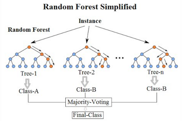
After the tree is made, we can make predictions by filtering down samples through the tree. The image at the top of this page shows a schematic of this. This is done for each sample (each row) in the dataset.7
function predict(tree::DecisionTreeClassifier, X::DataFrame)
    if tree.num_nodes == 0
        throw(NotFittedError(:tree))
    end
    probs = predict_prob(tree, X)
    return mapslices(argmax, probs, dims=2)[:, 1]
end

function predict_prob(tree::DecisionTreeClassifier, X::DataFrame)
    if tree.num_nodes == 0
        throw(NotFittedError(:tree))
    end
    probs  = zeros(nrow(X), tree.n_classes)
    for (i, xi) in enumerate(eachrow(X))
        counts = predict_row(tree, xi)
        probs[i, :] .= counts/sum(counts)
    end
    return probs
end


function predict_row(tree::DecisionTreeClassifier, xi::T ) where T <: DataFrameRow
    next_node = 1
    while !is_leaf(tree.binarytree, next_node)
        left, right = get_children(tree.binarytree, next_node)
        next_node = xi[tree.split_features[next_node]] <= tree.split_values[next_node] ? left : right
    end
    return tree.values[next_node]
end
The last major function is the calculation for the impurity based feature importances. For each feature, it can be defined as: the sum of the (weighted) changes in impurity between a node and its children at every node that feature is used to split. In mathematical notation:
\[FI_f = \sum_{i \in split_f} \left(g_i - \frac{g_{l}n_{l}+g_{r}n_{r}}{n_i} \right) \left( \frac{n_i}{n}\right)\]Where $f$ is the feature under consideration, $g$ is the Gini Impurity, $i$ is the current node, $l$ is its left child, $r$ is its right child, and $n$ is the number of samples.
The weighted impurity scores from find_better_split() need to be recalculated here.
function feature_importance_impurity(tree::DecisionTreeClassifier)
    if tree.num_nodes == 0
        throw(NotFittedError(:tree))
    end
    feature_importances = zeros(tree.n_features)
    total_samples = tree.n_samples[1]
    for node in 1:length(tree.impurities)
        if is_leaf(tree.binarytree, node)
            continue
        end
        spit_feature = tree.split_features[node]
        impurity = tree.impurities[node]
        n_samples = tree.n_samples[node]
        # calculate score
        left, right = get_children(tree.binarytree, node)
        lhs_gini = tree.impurities[left]
        rhs_gini = tree.impurities[right]
        lhs_count = tree.n_samples[left]
        rhs_count = tree.n_samples[right]
        score = (lhs_gini * lhs_count + rhs_gini * rhs_count)/n_samples
        # feature_importances      = (decrease in node impurity) * (probability of reaching node ~ proportion of samples)
        feature_importances[spit_feature] += (impurity-score) * (n_samples/total_samples)
    end
    # normalise
    feature_importances = feature_importances/sum(feature_importances)
    return feature_importances
end
There is another simpler method to calculate feature importance: shuffle (permutate) a feature column, and record how well the model performs.
Shuffling a column makes the values for each sample random, but at the same time keeps the overall distribution for the feature constant.
Scikit-learn has a great article on the advantages of this over impurity based feature importance.
(A perm_feature_importance() function is in the Classifier.jl file.)
BinaryTree
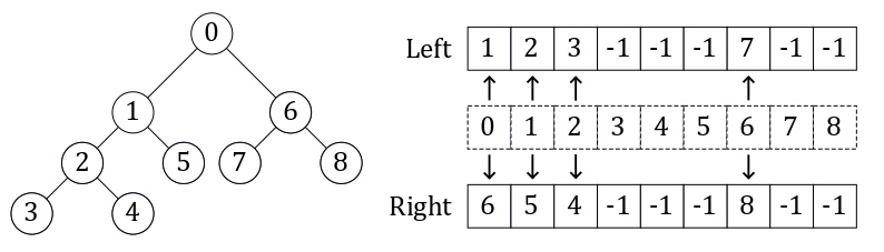
The most direct way to code a binary tree is to do so as a linked list. Each node is an object with pointers to its children. This was the method originally used in the FastAI course. The method that Scikit-learn uses, and that I chose to use, is to encode it as a set of two parallel lists. The image above shows an example of this representation. The index is the node ID, and the values in the left and right array are the node IDs (indexes) for that node’s children. If the value is -1, it means this node has no children and is a leaf. This method is more compact than the linked list, and has an O(1) look-up time for children given a node ID.
This is the smallest and simplest section, so I will present the entire code here without further explanation:
mutable struct BinaryTree
    children_left::Vector{Int}
    children_right::Vector{Int}
    BinaryTree() = new([], [])
end

function add_node!(tree::BinaryTree)
    push!(tree.children_left, -1)
    push!(tree.children_right, -1)
    return
end

function set_left_child!(tree::BinaryTree, node_id::Int, child_id::Int)
    tree.children_left[node_id] = child_id
    return
end

function set_right_child!(tree::BinaryTree, node_id::Int, child_id::Int)
    tree.children_right[node_id] = child_id
    return
end

function get_children(tree::BinaryTree, node_id::Int)
    return tree.children_left[node_id], tree.children_right[node_id]
end

function is_leaf(tree::BinaryTree, node_id::Int)
    return tree.children_left[node_id] == tree.children_right[node_id] == -1
end
Conclusion
I hope you enjoyed this post, and that it clarified the inner workings of a random forest. If you would like to know more, I again recommend Jeremy Howard’s FastAI course. He explains the rationale behind random forests, more on tree interpretation and more on the limitations of random forests.
What did you think of the top-down approach? I think it works very well.
In the future, I would like to investigate more advanced versions of tree ensembles, in particular gradient boosting techniques like CatBoost.
-
Don’t know what a sepal is? I didn’t either. It’s the outer part of the flower that encloses the bud. Basically it’s a leaf that looks like a petal. ↩
-
The F1 score balances recall (fraction of true positives predicted) with precision (fraction of correct positives). Guessing all true would have high recall but low precision. It is better to have both. $F1 =\frac{2}{\frac{1}{\text{recall}}+\frac{1}{\text{precision}}}$ ↩
-
The Julia convention is to not use underscores in the variable names. However I prefer this notation and use them extensively here. For example, I use
max_depthinstead ofmaxdepth. I think this makes the names clearer and easier to understand. Otherwise this disadvantages non-native English speakers. This is something I feel strongly about after having studied and worked in Europe where most of my colleagues spoke English as a second or third language. For example, for some languages it may be more natural to break “haskey” into “ha skey” or “hask ey” than the English “has key”. Using “has_key” eliminates this issue, but “haskey” is used in Base. ↩ -
Julia has no header guards like in C++. So if we included the “Utilities.jl” file here, as far as I know, it will recompile the “Utilities.jl” code, overwriting the old code in the process. But I could be wrong about that. ↩
-
Let the sample size be k and the total number of samples be n. Then the probability that there is at least one version of any particular sample is: \(\begin{align} P(\text{at least 1}) &= P(\text{1 version}) + P(\text{2 versions}) + .... + P(k \text{ versions}) \\ &= 1 - P(\text{0 versions}) \\ &= 1 - \left (\frac{n-1}{n} \right)^k \\\underset{n \rightarrow \infty}{lim} P(\text{at least 1}) &= 1 - e^{-k/n}\\\end{align}\).
For n=k, $P(\text{at least 1})\rightarrow 1-e^{-1} = 0.63212…$ ↩ -
Another way would probably be to determine the distribution of values e.g. linear, exponential, categorical. Then use this information to create a good feature range. ↩
-
The Python code used a more sophisticated method which grouped rows together in batches. This greatly sped up the Python code. But loop arrays are fast in Julia and I found no benefit to using batches here. ↩