Ping the world

I saw Erik Bernhardsson’s post on Ping the world on HackerNews and thought hey, I can do that! So I did the same from my home in South Africa. I had some difficulties, and encountered an amusing but scary story about a lawsuit involving a software glitch, a Kansas farm, and plenty of police officers and upset lovers. I’ll explain shortly. But first I’ll present my result after 60,000 successful random pings:

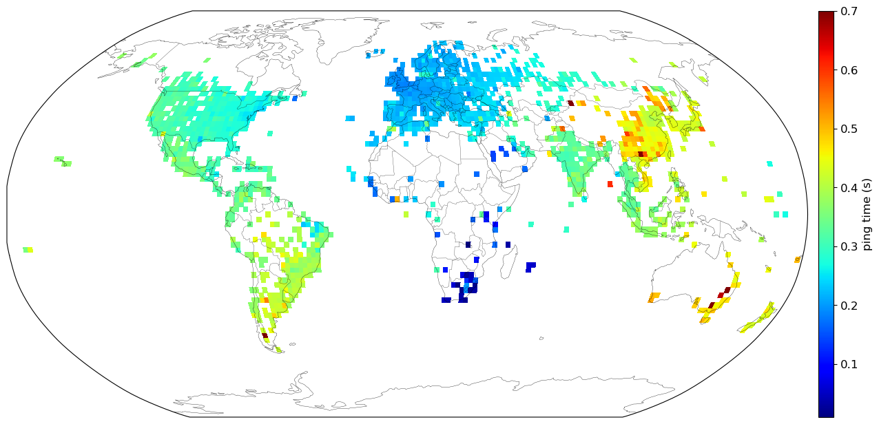
I’ve averaged the results to graticules of 2°×2°. There are plenty of blanks areas which correspond to low population densities like Siberia, the north and south poles and the Australian desert. Erik used a nearest neighbour approach to full in these gaps. I’ve left them blank because while a full map looks prettier, it doesn’t make sense to me to interpolate these large regions according to sparse data points.

This was a satisfying project to do, because after collecting raw data, it coalesced into a final result that makes sense. Closer countries tend to have faster round trip times, and the pings in South Africa are the fastest. I can ping most address in South Africa within 0.1 seconds and most addresses in the world within 0.7 seconds.

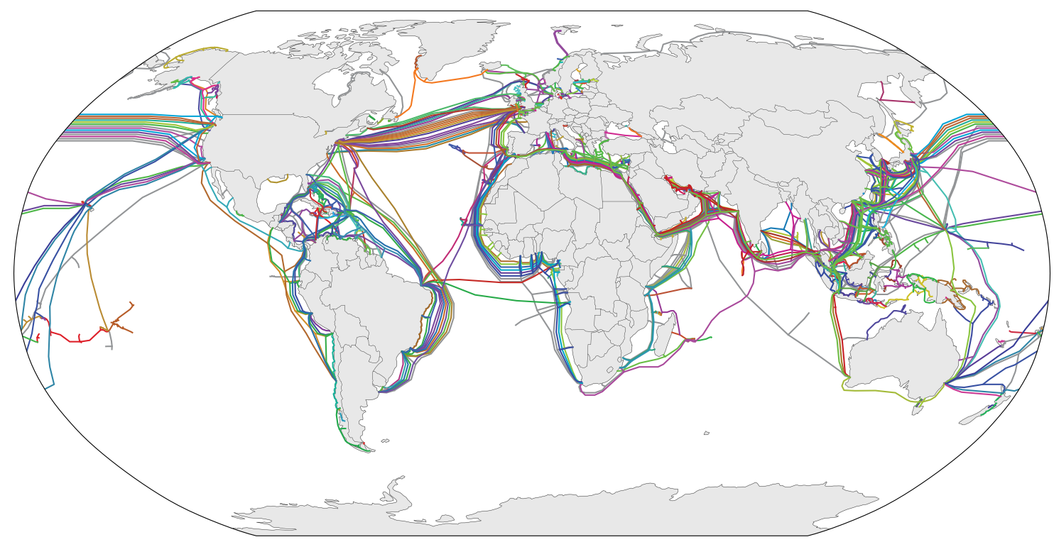
We can get even more insight by looking at a map of undersea cables, because physical distance is actually a proxy for cable distance. This is particularly important for Australia. Perth is roughly the same distance away from me as New Delhi, but there is no direct connection between South Africa and Australia like there is with India. Queries to Perth have to go through east Asia or Europe and North America. Hence queries to Australia are much slower than queries to India.

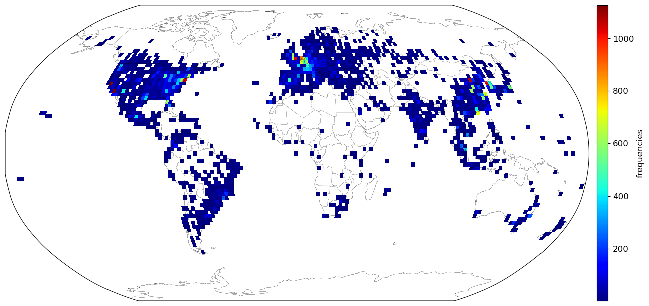
frequency of 60,000 ping locations — Frequency of pinged locations

These pings were done randomly but are not distributed equally around the world. There are clusters of high frequency in large metropolitans like New York, London and Seoul. Areas of low density populations are naturally empty, but on this Africa is an outlier. It is woefully underrepresented in the data even in regions of high population densities.

Pinging

I based my code on Erik’s. The code randomly assembles IPv4 addresses. Because we have practically run out of IPv4 addresses, there’s a good chance pinging a random one will work. About 86% of addresses will be in the geolocation IP database, and 10% will return a response. So to get 60,000 pings, I had to ping roughly 600,000 addresses.

The biggest bottleneck is unsuccessful pings. A good ping will be done in 0.3 seconds on average. But a bad ping will timeout after 4 seconds. To balance robustness with speed, I split pinging into 2 steps. Firstly I did one ping for a each address:

ping -n 1 <ip>

Then I went through the successful pings and got an average over four round trips:

ping -n 4 <ip>

Geolocating IPs

When I started this project, I copied Erik’s script and didn’t think much of the data source. This was a mistake. You should always think about the data. Here are lessons I learned the hard way in geolocating IP addresses.

1) It is an inexact science

Geolocating IPs is tricky. Don’t ever assume it to be accurate, because it’s not. There are large NGOs which manage IP blocks, so it is normally possible to get to a country level quite easily. After this, secondary data sources are used. This Wikipedia article suggests sources such as weather websites, pairing GPS information and data from Wifi hotspots.

I averaged my data over 2°×2°. This is equivalent to 220km×140km to 220km×220km depending on the latitude.¹ Even then, claiming a 200km radius of accuracy is probably pushing the limits of IP geolocation data.

2) Get the most recent data

Erik’s project is from 2015 and it uses a geolocation package last updated in 2015. I used this package from 2018. The data source is MaxMind’s Geolite2 database. To keep to the most up-to-date data, you can download the database directly from MaxMind and use the following code to get a reader of that database:

import geolite2
geo = geolite2.MaxMindDb(filename="path/to/GeoLite2-City.mmdb").reader()

However old data doesn’t affect the results much. Using an older database shifted points by 2° on average, well within a graticule’s limits.

3) IPv4 data is stored in blocks

The data in the database is stored in IPv4 CIDR blocks. Multiple IP addresses can map to the same block and therefore the same location. These blocks range in size from 1 IP address to millions. Again I will say, IPv4 geolocation data is not accurate.

Here is a concrete example. Consider the address 188.165.62.0/26. The numbers before the slash represent a 32 bit number written in groups of 256 ($256^4=2^{32}$). The number following the slash indicates the number of fixed leading bits. Here there are 26 fixed bits leaving $2^{32-26}=2^8=64$ variable bits. In other words, we can change the last number from from 0 to 63 and still be in the same block. Therefore all the IP addresses from 188.165.62.0 to 188.165.62.63 are part of the same block and will map to the same location. For the database I am using, these 64 addresses all map to a single location in central Amsterdam in the Netherlands. However they have an uncertainty of 500km so they could actually be spread all over the Netherlands.

The main database is in a custom format (.mmdb) which uses a binary search tree to speed up queries. Downloading the CSV version makes it more accessible for analytical queries. Then one can determine that it has 3.5 million entries for IPv4 blocks, but these represent 3.7 billion individual IP addresses. So on average, each block contains 1200 IP addresses.

Also, 3.7 billion is 85.9% of the total number of available IPv4 address of $2^{32} \approx 4.3$ billion. So a random IPv4 address has an 85.9% chance of being in the database.

4) Defaults

When I first made the frequency map, after something like 10,000 pings, I noticed something strange. The highest frequency location by far was a rural location in Kansas, USA. I had no idea why. Was there a secret massive server farm there? Some quick Googling led me to multiple articles involving a lawsuit with a Kansas farm being harassed by a continuous stream of law enforcement, upset lovers and self-proclaimed internet sleuths. A similar story surfaced about a house in my home country in Pretoria.

It turns out that the MaxMind database uses default locations at a country, state and city level. If an IPv4 address cannot be more precisely designated, it is assigned one of these default locations. Almost 60% of the database uses one of the default country locations. The USA default location alone has 1.17 billion IPv4 addresses assigned to it. This location used to be over a house, much to the occupants’ distress. Thankfully it has been moved slightly to sit over a lake. (The lawsuits were settled out of court.) Again I will say, IPv4 geolocation data is not accurate.

I chose to exclude any IP address which is sent to a default country location because I wanted my data to be accurate to a 2° level. Using the CSV files, it was very easy to extract these locations and blacklist them. (They are missing city, metro and subdivision labels.) If you want to shade a whole country the same colour, then it is alright to keep them.

After removing the defaults, this is what the frequency distribution for all 3.5 million unique IPv4 blocks looks like on a logarithmic scale, averaged to 1°×1° graticules:

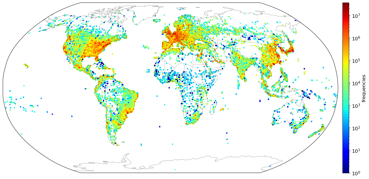
In general, this map corresponds well with population density data, except for underestimates in Africa. Tokyo is the highest density region, with 36 million IP addresses.

Conclusion

Hope you’ve enjoyed this and are ready to try it yourself!

The circle of latitude decrease in size with increasing latitude, so the graticules get smaller if you keep the angles constant. Have a look at a globe for a better idea. Each graticule will have a height of $\frac{\pi R}{N}$ but a varying width of $\frac{2\pi R}{2N}cos(\phi)$ where $\phi$ is the latitude. The area can be found by projecting it onto a cylinder. Hence the area will be $(\frac{\pi R}{N})(Rsin(\phi_1) - Rsin(\phi_2)) = \frac{1}{N}\pi R^2(sin(\phi_1) - sin(\phi_0))$ ↩

← Previous Post Next Post →